FSL Diffusion Toolbox Practical

In this practical we will walk you through the steps needed to prepare your diffusion data for analysis. We will also cover diffusion tensor model fitting and group analysis of DTI data using tract-based-spatial-statistics (TBSS).

Contents:

The FDT DTI Pipeline

The standard FSL diffusion processing pipeline

Diffusion Data

Familiarise yourself with diffusion data

TOPUP - Correcting for Susceptibility-induced Distortions

Identify EPI distortions and learn how to correct them using topup

EDDY - Correcting for Eddy Currents-induced Distortions

Identify Eddy-current induced distortions and learn how to correct them using eddy

DTIFIT - Fitting Diffusion Tensors

Fitting the diffusion tensor model to obtain scalar DTI maps (FA, MD) and fibre orientation information

TBSS - Tract-Based Spatial Statistics

Whole-brain voxelwise group statistics on DTI data

The FDT DTI Pipeline

Diffusion Data

In this first section of the practical we will familiarise ourselves with diffusion data. If you are comfortable with working with diffusion data, feel free to run through this section quickly or skip to TOPUP.

cd ~/fsl_course_data/fdt1/subj1_preproc

List this directory and you should see a set of files that are obtained from a typical diffusion MRI acquisition. This includes a dwidata file, as well as bvals and bvecs that contains the information on the diffusion-sensitising magnetic field gradients. Note that some nifti conversion tools will create bvals and bvecs information and some will not.

bvals contains a scalar value for each applied gradient, corresponding to the respective b-value. bvecs contains a 3x1 vector for each gradient, indicating the gradient direction. The entries in bvals and bvecs are as many as the number of volumes in the dwidata file. So the i^th volume in the data corresponds to a measurement obtained after applying a diffusion-sensitising gradient with a b-value given by the i^th entry in bvals and a gradient direction given by the i^th vector in bvecs. You can quickly see the contents of these two files, by typing cat bvals and cat bvecs, respectively.

Ensure you are comfortable with the term "shell".

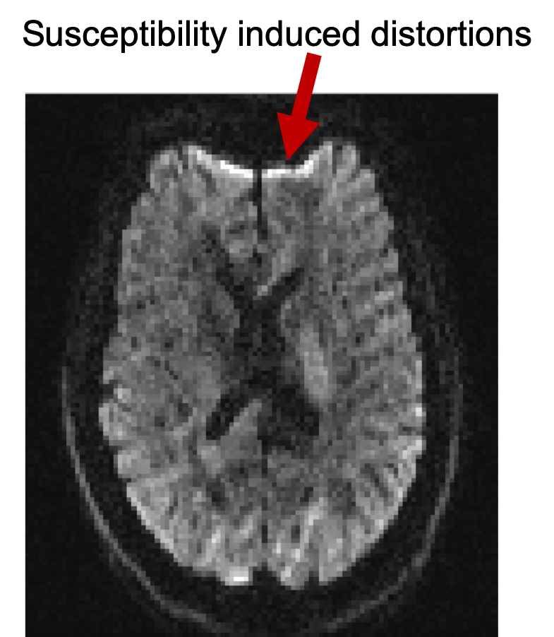
Bring up fsleyes and open b1500.nii.gz - you will need to reset the maximum display range to around 2000. This is the diffusion data of the b=1500 shell before correction for distortions and it is a 4D image. Turn on movie mode (). Look at the sagittal slice and note the movement between volumes caused by eddy current-induced distortions. The reason you see this as a "movement" is that each volume is associated with a different diffusion gradient, and hence different distortions. This particular subject happened to lie very still, but in general you would also see "movement" due to actual subject movement. Notice also the susceptibility-induced distortions at the frontal part of inferior slices.

Turn off movie mode, hide the b1500 overlay and open dwidata.nii.gz. Have a look through the different volumes (different "timepoints" in the 4D data) after setting the maximum display range to around 4000.

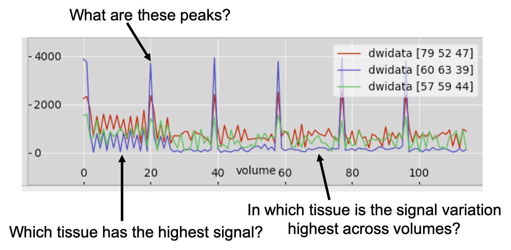
Now, let's have a look at all the data associated with a voxel. Choose a CSF voxel (e.g. [60, 63, 39]) and observe how the signal changes with gradient direction. To do that choose from the menu View > Time series. A new window will appear with a plot of the signal intensity at the chosen location for the different diffusion-weighted volumes. Notice the few high intensity values and the very low intensities in most of the datapoints. The former correspond to the b=0 images. The latter to diffusion-weighted images, for which maximal attenuation of the CSF signal has occurred.

Notice that the higher the b-value, the lower the signal. Can you identify time points that correspond to the three shells used in this acquisition? Check you are right by checking the bvals file (cat bvals).

Now, add to the plot the timeseries for a white matter voxel. To do that use the (+) button on the plot and choose a voxel in the corpus callosum (e.g. [57, 59, 44]). Can you tell and explain the differences in the data? Use (+) again and now choose a grey matter cortical voxel (e.g. [79, 52, 47]). Can you explain the differences?

Look again at the images. For volumes with diffusion gradients applied, see if you can work out the direction of the gradient. Remember that diffusion data appear darker in places where there is more diffusion along the gradient direction. You should be able to work out the gradient direction by looking at a diffusion weighted image, and comparing darker areas with your knowledge of white matter orientation. You can check if you are right - e.g for diffusion encoding direction for volume 4 (the fifth volume), type:

awk '{print $5}' bvecs

Diffusion MRI registration.

Typically the b=0 image or the FA image is used to register diffusion MRI data (i.e. to a structural scan or across subjects). Can you understand why this is? Why do we not use diffusion-weighted images?

TOPUP - Correcting for Susceptibility-induced Distortions

FSL wiki: https://fsl.fmrib.ox.ac.uk/fsl/fslwiki/topup

cd ~/fsl_course_data/fdt1/subj1_preproc

A minimum requirement for using topup for correcting distortions is that two spin-echo (SE) EPI images with different PE-directions have been acquired. The best is to acquire them with opposing PE-directions (i.e. A→P AND P→A or L→R AND R→L). An SE-EPI image is the same as a b=0 image acquired as a part of a diffusion protocol. Just as for fieldmaps this pair must be acquired at the same occasion as the full diffusion protocol and the subject must not leave the scanner in between and no re-shimming can be done.

Identifying susceptibility-induced distortions

From the dwidata choose a volume without diffusion weighting (e.g. the first volume). You can now extract this as a standalone 3D image, using fslroi. Figure out this command by yourself. Typing fslroi into the terminal will produce instructions on how to use fslroi. Call the extracted file nodif.

^*Reveal command

fslroi dwidata nodif 0 1

Open nodif in FSLeyes and have a look at different slices. Notice that as you go to more inferior slices, the frontal part of the brain starts to appear distorted (e.g. "squashed" or "elongated"). These distortions are always present in EPI images and are caused by differences in the magnetic susceptibilities of the areas being imaged.

Now open and superimpose in FSLeyes the image nodif_PA. This is an image without diffusion-weighting (i.e. b=0) of the same subject that has been acquired with the opposite PE direction (Posterior→Anterior). Switch on and off the visibility of this image to see how the distortions change sign between nodif and nodif_PA. Regions that are squashed in the first appear elongated in the second and vice versa. Unsurprisingly the areas that were very obviously distorted when viewed in the nodif image changes a lot as you switch back and forth between nodif and nodif_PA. Perhaps more disturbing is that some areas that didn't appear obviously distorted do too, meaning that these are also distorted, only not quite so obvious. For example look at the Cerebellum in a sagittal view at ~x=58 as you switch back and forth. We will correct these distortions by combining the two b=0 images using the TOPUP tool. We will then pass the results on to the EDDY tool where it will be applied to the correction of all diffusion data.

Running topup

First you need to merge the AP and PA images into a single image using fslmerge. Again, typing fslmerge into the command line will bring up helpful instructions. Merge the files along the 4th 'timeseries' axis. Call the merged image AP_PA_b0.

^*Reveal command

fslmerge -t AP_PA_b0 nodif nodif_PA

Then create a text file that contains the information with the PE direction, the sign of the AP and PA volumes and some timing information obtained by the acquisition. This file has already been created (acqparams.txt), and is a text-file that contains

0 -1 0 0.0759
0  1 0 0.0759

The first three elements of each line comprise a vector that specifies the direction of the phase encoding. The non-zero number in the second column means that is along the y-direction. A -1 means that k-space was traversed Anterior→Posterior and a 1 that it was traversed Posterior→Anterior. The final column specifies the "total readout time", which is the time (in seconds) between the collection of the centre of the first echo and the centre of the last echo. In the FAQ section of the online help for topup there are instructions for how to find this information for Siemens scanners.

The file should contain as many entries as there are volumes in the image file that is passed to topup.

We are now ready to run topup which we would do with the command:

topup --imain=AP_PA_b0 \
      --datain=acqparams.txt \
      --config=b02b0.cnf \
      --out=topup_AP_PA_b0 \
      --iout=topup_AP_PA_b0_iout \
      --fout=topup_AP_PA_b0_fout

applytopup --imain=nodif,nodif_PA \
           --topup=topup_AP_PA_b0 \
           --datain=acqparams.txt \
           --inindex=1,2 \
           --out=hifi_nodif

However, this will take too long to run so instead copy the "pre-baked" results into your working directory with:

cp pre_baked/topup_AP_PA_b0* .

There are four result files. topup_AP_PA_b0_fieldcoef.nii.gz contains information about the off-resonance field and topup_AP_PA_b0_movpar.txt specifies any movement between nodif and nodif_PA. Open FSLeyes and load topup_AP_PA_b0_fieldcoef.nii.gz. It looks like a low resolution fieldmap, and it contains the spline coefficients for the field that TOPUP has estimated. Close FSLeyes and re-open it, but this time take a look at the actual field (topup_AP_PA_b0_fout). Moreover, to check that TOPUP has done its job properly, load topup_AP_PA_b0_iout and compare its two volumes to those we provided as input (AP_PA_b0.nii.gz).

EDDY - Correcting for Eddy Currents

FSL wiki: https://fsl.fmrib.ox.ac.uk/fsl/fslwiki/eddy

We will first generate a brain mask using the corrected b0. We compute the average image of the corrected b0 volumes using fslmaths. Figure out the correct command, calling the output file hifi_nodif.

^*Reveal command

fslmaths topup_AP_PA_b0_iout -Tmean hifi_nodif

And then we use BET on the averaged b0. Again figure out the command and call the output file hifi_nodif_brain. Hint: create a binary brain mask, with a fraction intensity threshold of 0.2.

^*Reveal command

bet hifi_nodif hifi_nodif_brain -m -f 0.2

You can then use FSLeyes to ensure that bet has done a good job.

Running EDDY

Now we would typically run eddy, either through the FDT gui (by typing Fdt or Fdt_gui on a Mac), or with the command:

eddy --imain=dwidata \
     --mask=hifi_nodif_brain_mask \
     --index=index.txt \
     --acqp=acqparams.txt \
     --bvecs=bvecs \
     --bvals=bvals \
     --fwhm=0 \
     --topup=topup_AP_PA_b0 \
     --flm=quadratic \
     --out=eddy_unwarped_images \
     --data_is_shelled

In this command:

• dwidata is the full diffusion data (including b=0 volumes), all acquired with a Anterior→Posterior phase-encoding.
• The text-file index.txt contains a column of ones, one for each volume in dwidata, specifying that all volume were acquired with the parameters specified by the first row in acqparams.txt.
• topup_AP_PA_b0 was the name given as the --out parameter when we ran topup and will cause eddy to look for the files topup_AP_PA_b0_fieldcoef.nii.gz and topup_AP_PA_b0_movpar.txt.
• The parameters --fwhm=0 and --flm=quadratic specify that no smoothing should be applied to the data and that we assume a quadratic model for the EC-fields. These are our current recommendations and you are unlikely to ever have to use any other settings.
• Lastly, the --data_is_shelled flag is set to avoid the automatic checking on whether the data has been acquired using a multi-shell protocol (we already know that is indeed the case for this dataset).

As eddy performs a simultaneous registration of all volumes in the data set it is quite memory and CPU hungry. Therefore copy the pre-calculated results into your working directory with:

cp pre_baked/eddy_unwarped_images* .

You will find that eddy has produced three output files: eddy_unwarped_images.nii.gz, eddy_unwarped_images.rotated_bvecs and eddy_unwarped_images.eddy_parameters. The former of those is the "main result" and contains the data in dwidata corrected for susceptibility, eddy currents and subject movements.

We suggest that you load both b1500.nii.gz and eddy_unwarped_images_b1500.nii.gz into FSLeyes, set the maximum display range for both images to around 2000, make sure that the chain link icon () is turned on for both overlays in the Overlay List panel, then turn on movie mode (). The chain link option will group the display settings for the two selected images. By toggling the visibility of the top data set you can see the difference before and after eddy.

Data acquisition requirements for eddy (optional)

^*Read this either if you will be acquiring data on which you hope to run eddy, or if you want to to solidify your knowledge.

gps --ndir=64 --optws --out=my.bvecs

A note on quality control: EDDY QC

As we have seen, dMRI data can be affected by many hardware or subject-specific artefacts. If undetected, these artefacts can bias downstream analysis. Quality control is therefore very important - always look at your data! In large population studies, manual quality control may not be practical. A new FSL tool EDDY QC provides automatic quality control at both the single subject and group level. For more info see

FSL wiki: https://fsl.fmrib.ox.ac.uk/fsl/fslwiki/eddyqc .

DTIFIT - fitting diffusion tensors

cd ~/fsl_course_data/fdt1/subj1

The directory already contains bvals, bvecs, distortion-corrected data file named data and a brain mask named nodif_brain_mask. These are the four files that a standard FDT directory should be comprised of, before running dtifit or any further data analysis. The files are a sub-set of the data we have been working on so far, comprising only b=0 and b=1500 volumes. Here we select a single shell as the tensor is not a good model for multi-shell data.

select_dwi_vols \
    eddy_unwarped_images.nii.gz \
    bvals \
    dti_data \
    0 \
    -b 1500 \
    -obv eddy_unwarped_images.eddy_rotated_bvecs
  

You can run DTIFIT (the FSL diffusion tensor fitting program) in one of three ways, all described below. Choose one of these approaches:

1: Run DTIFIT on a FDT directory

Open the FDT GUI by typing Fdt (or Fdt_gui on a Mac), and select DTIFIT from the main menu (the button in the top that initially says PROBTRACKX).

You can run DTIFIT on a standard FDT directory by selecting the input directory (subj1 - go up one directory in the file browser to be able to select this) and then pressing Go. NB: When DTIFIT has finished running via the GUI, a small dialogue window will pop up saying Done! You must press Ok to close this window before closing the main FDT GUI otherwise you will recieve an error message (beware: this dialogue can pop up in a completely different and unexpected part of the screen).

2: Run DTIFIT by manually specifying the input files

Open the FDT GUI by typing Fdt (or Fdt_gui on a Mac), and select DTIFIT from the main menu (the button in the top that initially says PROBTRACKX).

You can select the input files manually by clicking Specify input files manually, then select the following files for the relevant tabs:

• Diffusion weighted data:   data
• BET binary brain mask:   nodif_brain_mask
• Output basename:   dti
• Gradient directions:   bvecs
• b values:   bvals

When you have entered all of the file name, press Go.

3: Call dtifit from the command line. Try to figure out this command yourself. Name the output files dti.

^*Reveal command

dtifit --data=data --mask=nodif_brain_mask \
  --bvecs=bvecs --bvals=bvals --out=dti

DTI output

When you have run dtifit using any of these three ways, load the anisotropy map dti_FA into FSLeyes

Add the principal eigenvector map to your display: File -> Add overlay from file -> dti_V1

FSLeyes should open the image as a 3-direction vector image (RGB). Diffusion direction is now coded by colour. For a more interpretable image, we can modulate the colour intensity with the FA map so anisotropic voxels appear bright. In the display panel () change the Modulate by setting to dti_FA. You may wish to adjust the brightness and contrast settings.

Change the Modulate by setting back to None, and then change the Overlay data type to 3-direction vector image (Line). Zoom in and out of your data. You should see clear white matter pathways through the vector field.

Finally, change the Overlay data type to 3D/4D volume. The image should now look quite messy - you are looking at the first (X) component (the first volume) of the vector in each voxel. The second and third volumes contain the Y and Z components of the vector.

Now load the Mean Diffusivity map (dti_MD) into FSLeyes. Change the minimum/maximum display range values to 0 and 0.001 respectively.

Compare the values of MD and L1 in CSF, white and gray matter.

^*What should I look at?

Next, load the secondary eigenvalue dti_L2 and see how L2 is lower in the white matter. Try also dti_L3. The contrast between white and gray matter is even larger, with much lower values being observed in the former. In contrast, L1, L2 and L3 do not vary that much in the gray matter (or in the CSF). These differences between L1, L2 and L3 give rise to diffusion anisotropy and lead to high FA values in the white matter and low FA in the gray matter. Keep in mind the diffusion tensor ellipsoid for a pictorial representation of the DTI eigenvalues.

We also have files named dti_V2 and dti_V3. What are these?

^*Answer

Visualising the tensor in fsleyes (optional)

In addition to displaying the principal eigenvector (dti_V1) of the tensor model fit, FSLeyes has the ability to display the full tensor model fit in each voxel. To do this, choose File -> Add overlay from directory and select the subj1 directory. Bring up the overlay display panel () and increase the tensor size and ellipsoid quality to improve visualization. You can now see the whole tensor elliposid colour-coded according to its PDD. In the overlay display panel, you can also choose to colour the ellipsoid using one of the loaded scalar maps (e.g., FA). Do that and select Colour Map -> Hot. It is now easier to see which white matter areas are more anisotropic than others and how this gets reflected by the shape of the tensor ellipsoid.

TBSS - Tract-Based Spatial Statistics

FSLwiki: https://fsl.fmrib.ox.ac.uk/fsl/fslwiki/TBSS.

So far, we have stepped through the steps required to pre-process a typical diffusion-weighted data. The final part of the tutorial focusses on running TBSS to compare FA values between two groups of participants.

We will now run a TBSS analysis of a small dataset - 3 young people (mean age 25) and 3 older people (mean age 65). We will attempt to find where on the tract skeleton the two groups of subjects have significantly different FA.

1. Creating FA data from a diffusion study

We have already created the FA images from the 6 subjects, using dtifit.

cd ~/fsl_course_data/fdt1/tbss

Remember that all of the main scripts (until you reach the randomise stage near the end) need to be run from within this directory.

LOOK AT YOUR DATA

• Open one image with FSleyes to get a feel for the raw data quality and resolution. You may need to adjust the intensity display range. Look at the image histogram (View -> Histogram).
• Run slicesdir *.nii.gz and open the resulting web page report; this is a quick-and-dirty way of checking through all the original images.

2. Preparing your FA data for TBSS

We must first run an additional pre-processing script which will erode your FA images slightly to remove brain-edge artifacts and zero the end slices (again to remove likely outliers from the diffusion tensor fitting). Type:

tbss_1_preproc *.nii.gz

The script places its output in a newly-created sub-directory called FA. It will also create a sub-directory called origdata and place all your original images in there for posterity.

LOOK AT YOUR DATA

Check the images created in the FA directory. The tbss_1_preproc script will have re-run slicesdir on the preprocessed FA maps - open this report (you can find it in FA/slicesdir/index.html) and compare it to the slicesdirreport you created earlier.

3. Registering all the FA data

The next TBSS script runs the nonlinear registration, aligning all the FA data across subjects. The recommended approach is to align every FA image to the FMRIB58_FA template. This process can take a long time, as each registration takes around 10 minutes. You can easily speed this up if you have multiple computers running cluster software such as SGE (Sun Grid Engine). To save time, we have pre-computed all the alignments for you, so instead of running the TBSS script tbss_2_reg, make sure you are still in the directory one level above FA, and run:

cp precomputed_registration/* FA

This puts the necessary registration output files into FA, as if you had run the registration yourself.

4. Post-registration processing

Before reading this section, start the next script running so that you can read what's going on while it runs (it will take about 5 minutes):

tbss_3_postreg -S

The previous script (tbss_2_reg - we ran this for you) only got as far as registering all subjects to the chosen template. The tbss_3_postreg script applies these registrations to take all subjects into 1x1x1mm standard space.

The script then merged all of the subjects' standard space nonlinearly aligned images into a single 4D image file called all_FA, created in a new subdirectory called stats. The mean of all FA images is created, called mean_FA, and this is then fed into the FA skeletonisation program to create mean_FA_skeleton.

Once the script has finished running, check that the mean FA image looks reasonable, and is well aligned with the MNI152 image:

cd stats
fsleyes -std1mm mean_FA -cm red-yellow -dr 0.2 0.6 &

As you move around in the image you should see that the mean FA image is indeed well aligned to standard space and corresponds to white matter in the MNI152 image. Remove these images (Overlay -> Remove all), then open the aligned FA maps for all subjects and the mean FA skeleton (File -> Add overlay from file, and select all_FA and mean_FA_skeleton). Change the colour map for mean_FA_skeleton to Green, and the display range to 0.2 - 0.6.

Select all_FA and turn on the movie loop (); you will see the mean FA skeleton on top of each different subject's aligned FA image. If all the processing so far has worked, the skeleton should look like the examples shown in the lecture. If the registration has worked well you should see that in general each subject's major tracts are reasonably well aligned to the relevant parts of the skeleton.

What happens if we set the skeleton threshold lower than 0.2? To do this in FSLeyes, change the lower of the display range settings.

^*Answer

5. Projecting all pre-aligned FA data onto the skeleton

The last TBSS script carries out the final steps necessary before you run the voxelwise cross-subject stats. It thresholds the mean FA skeleton image at the chosen threshold:

If you're still in the stats directory:

cd ..

Then:

tbss_4_prestats 0.3

This takes 4-5 minutes to run; read the rest of this section while it's running (if you can't make much sense of it, don't worry - it's described in more detail in the paper!).

The thresholding creates a binary skeleton mask that defines the set of voxels used in all subsequent processing.

Next a "distance map" is created from the skeleton mask. This is used in the projection of each subject's FA onto the skeleton; when searching outwards from a skeleton voxel for the local tract centre, the search only continues while the distance map values keep increasing - this means that the search knows to stop when it has got more than halfway between the starting skeleton point and another separate part of the skeleton.

Finally, the script takes the 4D pre-aligned FA images in all_FA and, for each "timepoint" (subject ID), projects the FA data onto the mean FA skeleton. This results in a 4D image file containing the (projected) skeletonised FA data. It is this file that you will feed into voxelwise statistics in the next section.

Once the script has finished, cd into stats and have a look at all_FA_skeletonised in FSLeyes - turn on movie mode to see the different timepoints of the skeletonised data.

6. Voxelwise statistics on the skeletonised FA data

The previous step resulted in the 4D skeletonised FA image. It is this that you now feed into voxelwise statistics, that, for example, tells you which FA skeleton voxels are significantly different between two groups of subjects.

The recommended way of doing the stats is to use the randomise tool. For more detail see the Randomise manual. Before running randomise you will need to generate design matrix and contrast files (e.g., design.mat and design.con). We will use the Glm GUI to generate these. Note that the order of the entries (rows) in your design matrix must match the alphabetical order of your original FA images, as that determines the order of the aligned FA images in the final 4D file all_FA_skeletonised. In this case the order was: 3 young subjects and then 3 older subjects. Start the GUI:

cd stats
Glm

Change Timeseries design to Higher-level / non-timeseries design. Change the # inputs to 6 (you may have to press the enter key after typing in 6) and then use the Wizard to setup the Two-groups, unpaired t-test with 3 as the Number of subjects in first group (Note that the order of the subjects will be important in this design). Reduce the number of contrasts to 2 (we're not interested in the group means on their own). Finally, save the design as filename design, and in the terminal use less to look at the design.mat and design.con files.

You are now ready to run the stats. Because this reduced dataset only contains 6 subjects, only 20 distinct permutations are possible, so by default randomise will run just these 20. Again, because this tiny dataset has so few subjects the raw t-stat values will not be very significant - so let's try setting a cluster-forming t threshold of 1.5 (in "real" datasets we would normally recommend using the --T2 option for TFCE instead of cluster-based thresholding):

randomise -i all_FA_skeletonised -o tbss \
  -m mean_FA_skeleton_mask -d design.mat -t design.con -c 1.5

Contrast 1 gives the young>older test. The raw unthresholded tstat image is tbss_tstat1 and the corresponding (p-values corrected for multiple comparisons) cluster image is tbss_clustere_corrp_tstat1.

Thresholding clusters at 0.95 (corresponding to thresholding the p-values at 0.05, because randomise outputs p-values as 1-p for convenience of display - so that higher values are more significant) shows a few areas of reduced FA in the older subjects. The following shows unthresholded t-stats in red-yellow and thresholded clusters in blue:

fsleyes -std1mm mean_FA_skeleton -cm green -dr .3 .7 \
  tbss_tstat1 -cm red-yellow -dr 1.5 3 \
  tbss_clustere_corrp_tstat1 -cm blue-lightblue -dr 0.949 1 &

Look at the histogram of tstat1; it is clearly shifted to the right, suggesting a global decrease in FA with aging (you may need to change the number of histogram bins to see this easily).

^*Displaying "fattened" results

tbss_fill tbss_clustere_corrp_tstat1 0.95 \
      mean_FA tbss_clustere_corrp_tstat1_filled
    

The End.