FEAT 1 Practical

This tutorial leads you through a standard single-subject analysis with FEAT. There may be moments when you are waiting for programs to run; during those times take a look at the FEAT manual (in particular go to the User Guide and look at the FEAT in Detail section). We also suggest that you do read it carefully after the course, before using FEAT for analysing your own data.

Contents:

Example real fmri dataset

Perform a full first-level analysis of a single subject in a memory encoding experiment.

Featquery

Use featquery to interrogate results of the previous analysis and extract ROI measurements.

Quality checks

Make sure to look at all of the stages of the analysis to ensure that they have all worked.

Optional: Sorting your data

Use some scripting to organise the input files for your analysis.

Example real fmri dataset

cd ~/fsl_course_data/feat1/sub-001

The dataset func/sub-001_task-memory_bold.nii.gz is from an encoding memory task. The TR is 3.0 seconds. The experiment had a blocked design of alternating blocks of two conditions:

1. Familiar images: Here the participant was presented with images from a set previously seen outside the scanner.
2. Novel images: Here the participant was presented with never before seen images.

Before scanning, participants were presented 8 times with 8 images ("familiar" images) and tested to ensure images had been encoded. During the experiment, participants were presented with 12 blocks (6 familiar, 6 novel) containing colour images of landscapes or animals. Each block lasted 30 seconds, and contained 8 images (4 animals, 4 landscapes). Images were presented in a pseudorandom order. The participant was asked to indicate whether each image contained an animal, and to try and remember the image. The blocks alternated with periods of rest. The stimulus onset file has been provided.

With this task, we are interested to determine: (a) where novel information is processed relative to baseline, (b) where familiar information is processed relative to baseline, and (c) where novel information is processed relative to familiar information.

So, let us get started with the analysis.

Feat &

(Type Feat_gui & if you are on a Mac).

Data

Feat starts by displaying the Data tab. Load the 4D data and check the number of volumes and TR are correct. Hint.

The High pass filter cutoff is preset to 100secs. This is chosen to remove the worst of the low frequency trends, and is also long enough to avoid removing the signal of interest. In general you need to ensure that this is not set lower than your maximum stimulation period. For blocked designs, a good rule of thumb is to choose a minimum cut-off that is at least as long as a full cycle in your model, in seconds. However, leave it at the default for now and we'll come back to it when we have specified the design.

Pre-stats and Stats

Press the Pre-stats tab to look at the preprocessing steps. Select B0 unwarping and specify the fieldmap images and settings (parameters can be found in ~/fsl_course_data/feat1/sub-001/fmap/sub-001_params.txt). All the other default pre-processing steps are fine for this dataset. Hint.

Setting up the design matrix

Select the Stats tab and press Full model setup to setup the GLM details. Specify the EVs for our two conditions using the 3-column format under Basic Shape and the timing files already organised into the appropriate format. Hint.

For now, unset Add temporal derivative. We would normally recommend leaving it set (and we will come back to set it) but in order to obtain a very simple initial design we will unset it for now.

Setting up contrasts

Now set up the Contrasts (click on the Contrasts & F-tests tab). Your contrasts of interest at this level have to do with the experimental design within an individual. Remember that fMRI is all about contrasting signals in order to isolate some mechanism of interest.

Set the contrasts to answer questions (a), (b), (c), (d) and (e) below. Hint.

(a) where is novel information is processed relative to baseline?
(b) where is familiar information is processed relative to baseline?
(c) where is novel information processing greater than familiar information processing?
(d) where is novel information processing less than familiar information processing?
(e) where do we see mean activation across novel and familiar information relative to baseline?

If you haven't already, click on Hint above to check your model design.

Next set up an F-test to investigate whether there is significant activation by novel AND/OR familiar images. Hint.

Press View design. Make sure you understand the resulting design matrix.Hint.

Temporal derivatives

Now, return to the EVs tab and FOR BOTH EVs select Add temporal derivative.

Press View design again. You now see 4 columns with columns 1 and 3 being the same as before and column 2 and 4 being "new". These are the temporal derivatives that are used to correct for timing errors caused either by slight experimental errors in synchronising the times of the scanner with the stimulus presentation and/or inter-subject differences in the delay inherent in the HRF. Now press "Done" and dismiss the view of the design matrix.

Now we will return to the issue of High pass filtering now we know the design (and with that the expected frequency content of the signal we expect/hope to see). Press the Data-tab to make sure that High pass filter cutoff (s) is set to 100. Next press the Misc-tab where there will be a button saying Estimate High Pass Filter. Press this button and then go back to the Data-tab to see what has happened. This should now have changed to 90 seconds. FSL has calculated this for you by analysing the frequency content of the design and then selected a cutoff so that 90% of our expected signal is still in the data after filtering. (N.B. that it is just a fluke that 90% happened to translate into 90 seconds in this particular case)

Look at the Post-stats section. Cluster-based thresholding will be carried out. Check the Z threshold is set to 3.1. All other defaults are fine.

Registration

Select the Registration tab. Specify the Main Structural image and use the BBR method. Leave the default Standard Space image and use 12DOF. The more accurate nonlinear registration is normally recommended for registration to MNI space by selecting the "nonlinear" option, but we use linear here as it is faster for this practical. Hint.

Go!

You are now ready to run FEAT. Press Go. A web browser should appear, and as FEAT completes the different stages of processing, you will see messages appear in the Log section. Whether the web browser (and indeed the FEAT GUI) is left displayed or is closed, FEAT will continue to run in the background. For now, leave the web browser open so that you can monitor FEAT's progress. FEAT will take approximately 20 minutes to complete.

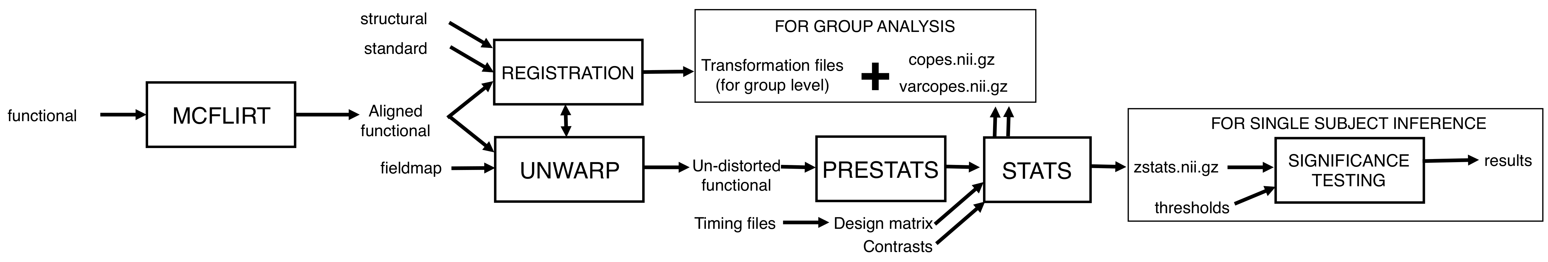
While you wait

Take a look at the flow diagram below that summarises all of the steps that you just set up in FEAT. Hopefully it will help you to see the big picture, and avoid getting bogged down in the details:

Whilst FEAT is running, run FSLeyes to have a quick look at the different images mentioned above: start by looking at anat/sub-001_T1w_brain.nii.gz, and then view func/sub-001_task-memory_bold.nii.gz.nii.gz. Note that when viewing the 4D image you can see the image time series as a movie by pressing on the movie icon (), and you can also see time series plots by pressing View > Timeseries.

Create a mask to probe statistics

Whilst FEAT is still running, we will now use FSLeyes to create a mask in standard space that will be used later to find out about activation statistics from within the mask.This might be important if you want to conduct a detailed analysis of a specific area of the brain, i.e. to plot it against a specific behavioural variable outside of FEAT. An alternative method to create a mask was explained in the Registration practical.

1. Reopen FSLeyes and load the standard space template image $FSLDIR/data/standard/MNI152_T1_2mm ($FSLDIR is an environment variable indicating the directory in which FSL is installed, you can type echo $FSLDIR to see what this is set to). Inside FSLeyes you can use the File -> Add standard menu option to find these standard space images quickly.
2. Open the atlas panel via Settings -> Ortho View 1 -> Atlas panel, and enable the Harvard-Oxford Cortical, Harvard-Oxford Subcortical and Juelich Histological atlases. Move the cursor around a little in the standard brain and see how the labels and numbers in the atlas tool window change. If you have a favourite part of the brain and you happen to know where it is you can move the cursor there and see if the atlas tool agrees with you.
3. Now select the Atlas search tab in the atlas panel, and choose the Harvard-Oxford Subcortical from the list on the left. You will now see a list of all the structures in that atlas on the right.
4. Type hippocampus in the text box above the structure list to filter the structures that are shown. Click the check box next to Right Hippocampus.
5. You will notice that in the FSLeyes overlay list, an image has been added with name corresponding to the region you just selected. If you move the cursor around within the brain you will notice its intensity values in changing between 0 and 100. These values reflect the probability that a given voxel (cursor position) is indeed part of that structure.
6. Press the save icon () next to the image harvardoxford-subcortical/prob/Right Hippocampus in the overlay list and save the image to a file called right_hippocampus.

7. What we will do next is to create a mask which has the value 1 for each voxel that has a 50% or greater chance of belonging to the right hippocampus. We do this by typing (in the terminal window):

   fslmaths right_hippocampus -thr 50 -bin right_hippocampus_mask

   The end result of this is a file named right_hippocampus_mask.nii.gz that we will later use as a mask to plot time-series of our results. To check the mask you have just created in FSLeyes, type

   fsleyes -std right_hippocampus_mask -cm red

   and have a look.

Look at the EV specification

Take a look at the files that we used to specify our design, i.e. sub-001_task_familiar_events.txt and sub-001_task_novel_events.txt. These are located in ~/fsl_course_data/feat1/sub-001/func/ We do this by typing (still in the terminal window):

more sub-001_task_familiar_events.txt

The more command will show you the contents of the file (type q to quit if the terminal doesn't give you your prompt back). Once you've finished looking at sub-001_task_familiar_events.txt, type more sub-001_task_novel_events.txt to look at the timing information for the novel images.

While FEAT is running, it will display STILL RUNNING in the main FEAT report page, which is replaced by Finished at ... when it is done.

Once FEAT has finished, look carefully at the various sections of the web page report, including motion correction plots in the Pre-stats section, the colour-rendered activation images and timeseries plots in the Post-stats section, and the Registration results. Note that if you click on the activation images you get a table of cluster co-ordinates. If your FEAT analysis is taking a long time, you can look at the report.html of another subject that we have already run for you in ~/fsl_course_data/feat1/prebaked/sub-002

Also look at the contents of the FEAT directory.

Looking ahead: The output of multiple lower level FEAT analyses (across mutliple subjects or sessions) will form the input to the higher level FEAT analyses, which we will work on in feat2 and feat3 practicals.

Featquery

Featquery allows you to calculate certain statistics, either at a voxel of interest, or averaged over a region of interest using a mask. We will use the standard-space mask that we created earlier. Start up Featquery from the terminal:

Featquery &

(or Featquery_gui & if you are on a Mac).

Select the .feat directory created in your first analysis on the fmri dataset, called fmri.feat unless another output name was specified. If your FEAT has still not finished running, you can use another subject that we have already run for you in ~/fsl_course_data/feat1/prebaked

Featquery automatically reads the FEAT directory and gives you the appropriate options as to which statistics you can choose to investigate.

1. Select the following statistics for the contrast that looks at activation for novel (i.e. the [1 0] contrast), the contrast that looks at activation for familiar (i.e. the [0 1] contrast) and the contrast that looks at activation for novel images over and above familiar (i.e. the [1 -1] contrast):
   • stats/cope (unthresholded contrast of parameter estimate)
   • stats/tstat (unthresholded t statistics)
   • stats/zstat (unthresholded z statistics)
   • thresh_zstat (thresholded z statistics)
   
   

   Note that the numbers you need to select will depend on the order you specified your contrasts earlier.

2. In the Input ROI selection panel, enter the mask that you created earlier (i.e. right_hippocampus_mask.nii.gz) as the Mask Image (note - Featquery can take either a standard-space mask OR a lowres one in the original dataspace OR a mask in the space of the structural image)
3. In the Output options section, select the Convert PE/COPE values to % option
4. Select the Do not binarise mask (allow weighting) option
5. Press Go and a web browser showing the estimated statistics should popup shortly (possibly a minute or two if things are busy).

The resulting web page will contain a table summarizing each of the statistics that you asked Featquery to report on in step 1. The first column gives the statistic name. The second column gives the number of non-zero voxels in the mask. The next group of columns gives a summary of the distribution of values within the mask. Plots of the timeseries at the maximum z-stats are available by clicking the link labeled "Masked time series plot" just below the image of the mask at the top of the page.

Looking ahead: Featquery can also be extended to probe the group level results. Multiple lower level FEATs can be input, and as long as registration has been run on all subjects, you can input a standard space mask, which Featquery will transform into the indiviudal subject space for you.

Quality checks

It is crucial to check your results to make sure the preprocessing, registration and model fit stages have gone well.

When you are doing your own experiments, you should look through every first level analysis you run at this stage to make sure you have selected the appropriate parameters for your design. We have already done that for you here, but we have selected some subjects for you to pay special attention to.

Registration check

Change directory into the 'prebaked' directory, where some FEAT analyses have been run for you for some other participants.

cd ~/fsl_course_data/feat1/prebaked

For subjects sub-002 and sub-016 please look at the FEAT Registration page. Check the alignment of the brain edges and ventricles at each stage of the registration, and check the unwarping stages. Are there any particularly problematic areas of the brains? Which subject has better registration to standard space? Are these registrations adequate for group analysis?

Preprocessing checks

For the same subjects, take a look at the Pre-stats page of the FEAT report and check for motion. Which subject has less motion? Please note there is no simple rule of thumb for defining too much motion. However, you might want to have a closer look at any subjects with motion over 1 voxel to assess the quality of the preprocessing. Would you want to re-run any of these subjects based on what you see? Why or why not?

Model fit check

For subjects sub-002 and sub-016, look at the Stats and Post-stats pages of the FEAT report and check the quality of the model fit for contrast of interest - novel > familiar [1 -1]. Which of these subjects has a better model fit for this contrast? How can you tell? Is there anything particularly noticable in the Post-stats page of either of the subjects?

Optional: Sorting your data

Set yourself up

In the present dataset, we prepared the fieldmaps and structural scans for you. We also organised the filenames in a consistent way. Normally there is no such consistent naming convention for files obtained directly from the scanner/reconstruction programme. The scanner typically names files according to some convention of scan order, and what happened during the scanning session (e.g. if any sequences needed to be re-run). These names can get confusing quickly, so it can be helpful to rename files in a consistent way from the very beginning yourself.

To do so, we recommend following the guidelines of the Brain Imaging Data Structure (BIDS). BIDS essentially organises data into separate folders for each subject, with separate subfolders for structural data (sub-001/anat), functional data (sub-001/func), fieldmaps (sub-001/fmap) and diffusion data (sub-001/dwi).

This section is intended to give you a bit more practice in the unix environment and to illustrate how to organise/check your data. As is the case for all commands, if you do not know the usage for a command, you can always just type the command into a terminal and get some help. Open a terminal and type cp or cp --help then press return to see what happens.

It is a good idea to think about how to organise your data ahead of time, so that you have identical directory structures for each subject, starting with the file you create when you load your raw data from the scanner (and sometimes need to convert it into NIFTI format). You can zero pad your numbers to help with this: e.g. if you have 5 subjects, don't name the files 1 2 3 4 5, but instead name them sub-001 sub-002 sub-003 sub-004 sub-005. You should use this structure as soon as you get your raw data.

Rename your images

Change directory to 'originals':

cd ~/fsl_course_data/feat1/originals/sub-020

Here we have the raw files for subject 020. We will practice some organisation. You can, of course, organise data from anywhere on your machine if you use pathnames in your commands. When you are learning, though, you might find it easiest to create a working copy of all the files within the directory you are reorganising, just in case:

You can copy and save an image under a new name with one easy command:cp images_2_ep2d_axial.nii.gz sub-020_task-X_bold.nii.gz

Now take a look at the other files in this directory, use FSLeyes or fslhd to identify the scans. Extend the cp example above to rename these scans appropriately so that you end up with your structural, functional, and fieldmap images renamed.

Make a new directory: mkdir raw You can move all the raw files you just renamed into that directory using:mv images* raw/ (the asterisk means that all files starting with images will be selected).

You might run into instances where you just want to rename and replace the same images for all of your subjects (if you want to copy rather than replace files, just use cp instead of mv). Do not run these commands, just take a look at them in case it might be helpful in the future. If you want to do the same thing to lots of files you can either

Run the command separately for each subject: mv images_2_ep2d_axial.nii.gz raw/sub-020_task-X_bold.nii.gz

Write a 'for loop'. Let's say you have 5 subject directories: sub-001 sub-002 sub-003 sub-004 005, and you need to rename the EPI images for all subjects. The example code below could be run from the directory that contains all the subject directories to rename your functional image:

for subject in sub-001 sub-002 sub-003 sub-004 sub-005; do
	mv ${subject}/images_2_ep2d_axial.nii.gz ${subject}/func/${subject}_task-X_bold.nii.gz
done

The for loop can save you a lot of time in many situations (for example, if you want to select multiple datasets in FEAT, you can write a loop that will call all the directories rather than having to select each of them by hand), so it's worth familiarizing yourself with these commands.

Since you set up your data nicely, you can write an even better for loop which allows you to refer to the structure of the directory names instead of listing them all. This would also change all file names in the same command:

for subject in sub-0??; do
	mv ${subject}/images_2_ep2d_axial.nii.gz ${subject}/func/${subject}_task-X_bold.nii.gz
	mv ${subject}/images_95_field.nii.gz ${subject}/fmap/${subject}_magnitude1.nii.gz
	mv ${subject}/images_mpr.nii.gz ${subject}/anat/${subject}_T1w.nii.gz
done

Once you have a consistent system for identifying data and scans, you can set up a group level analysis with less room for error.

The End.