Structural Analysis Practical

In this practical you will learn to use the main tools for structural analysis: FAST (tissue-type segmentation), FIRST (sub-cortical structure segmentation) and FSL-VBM (local grey matter volume difference analysis). In addition there are several optional extensions, including BIANCA and SIENA, that will be relevant to those with interests in particular types of structural analysis. We advise people to pick and choose based on their own particular interests; everyone should do FAST, but after that the parts are quite separate and can be done in any order (e.g. people particularly interested in VBM might want to do that before the section on FIRST).

Contents:

FAST

Perform tissue-type segmentation and bias-field correction using FAST.

FIRST

Use FIRST for segmentation of sub-cortical structures. Introduces basic segmentation and vertex analysis for detecting group differences.

FSL-VBM

Perform an FSL-VBM (voxel-based morphometry) analysis for detecting differences in local grey matter volume.

Optional extensions:

BIANCA

Use BIANCA to detect white matter lesions.

SIENA

Use SIENA for detecting global grey-matter atrophy in longitudinal scans.

SIENAX

An introduction to the cross-sectional version of SIENA.

FIRST Revisited

Looking at the "uncorrected" FIRST outputs.

Multi-Channel FAST

An introduction to the multi-channel version of FAST - for use with multiple acquisitions (e.g. T1-wt, T2-wt, PD, ...).

FAST

In this section we will segment single T1-weighted images with FAST and look at how to quantify the grey matter volume and amount of bias field present.

cd ~/fsl_course_data/seg_struc/fast

FAST Input Preparation - BET

To begin with we will prepare data for FAST; this requires running BET for brain extraction. In addition, just for this practical, we will also extract a small ROI containing a few central slices so that FAST only takes a minute to process the data, instead of 10-15 minutes for a full brain.

Run BET on the input image structural to create structural_brain (type Bet for the GUI [Bet_gui on a Mac], or bet for the command-line program).

Look at your data

View the output to check that BET has worked OK (e.g. change the colourmap for structural_brain to say Red-Yellow):

fsleyes structural structural_brain &

Back in the terminal, create a cut-down version (containing a few central slices) of the brain-extracted image using the region-of-interest program fslroi. This will let you try out some of the FAST options without having to wait more than a minute each time.

fslroi structural_brain structural_brain_roi 0 175 0 185 100 5

Load structural_brain_roi into FSLeyes to see the cut-down image. See how few slices are left. Leave FSLeyes open for the moment.

Image with Bias Field

You will also find an image in this directory called structural_brain_7T.nii.gz which contains a section of the same brain acquired on a 7 Tesla scanner with a different bias field or inhomogeneity, and a cut-down version structural_brain_7T_roi.nii.gz.

Add structural_brain_7T_roi.nii.gz to the already open FSLeyes (or open a new one and load structural_brain_roi first) and then look at the difference between these images. Note how both grey matter and white matter are darker in the left anterior portion of the 7T image.

FAST - Single Channel Example

Run FAST (separately) on both structural_brain_roi and structural_brain_7T_roi. Use the GUI (Fast [or Fast_gui on a Mac]) and turn on the Estimated bias field button (which saves a copy of the bias field) and Restored input button (which corrects the original image with the calculated bias field). For both images also open the Advanced Options tab and change the Number of iterations for bias field removal to 10 to account for the strong bias fields in both cases.

Finally, don't forget to check that the output name is different for the two runs (structural_brain_roi and structural_brain_7T_roi)! Once this is set up press Go for both - they should only take a minute to run.

Bias Field Correction

Now let's look at the bias field outputs - structural_brain_roi_bias and structural_brain_7T_roi_bias (these are FAST's estimates of the bias fields). View these in FSLeyes and set the display ranges to be equal for both images (e.g. 0.6 to 1.4). Notice how different the two bias fields are.

Open both of the *_seg.nii.gz output segmentations in FSLeyes. Try using different colour maps for the segmentations when viewing the results. You can now see how a different bias field can alter the segmentation of the image.

Partial Volume Segmentation

Now let's look at the partial volume segmentations. View the different outputs in FSLeyes by first loading structural_brain_roi_restore, then loading the PVE (Partial Volume Estimate) images as overlays, adjusting the overlay opacity as necessary. Note that you can tell FSLeyes what colourmaps and intensity ranges to use from the command line:

fsleyes structural_brain_roi_restore \
  structural_brain_roi_pve_0 -cm green -dr 0.5 1 \
  structural_brain_roi_pve_1 -cm blue-lightblue -dr 0.5 1 \
  structural_brain_roi_pve_2 -cm red-yellow -dr 0.5 1 &

Identify which PVE component is the grey matter. Choose a voxel on the border of the grey matter and look at the values contained in the three PVE components. The values represent the volume fractions for the 3 classes (GM, WM, CSF) and should add up to one. Now pick a point in the middle of the grey matter and look at the three values here.

The PVE images are the most sensitive way to calculate the tissue volume which is present. For example, we can find the total GM volume with fslstats by doing:

fslstats structural_brain_roi_pve_1 -M -V

The first number reported by fslstats gives the mean voxel GM PVE across the whole image, the second is the number of voxels and the third number gives the total volume of the image (in mm³) ignoring all voxels which are zero. Multiplying the first and third numbers together will give the total GM volume in mm³ (for more details on fslstats just type fslstats to see its usage description).

FIRST

In this section we lead you through examples of subcortical structure segmentation with FIRST, and some post-fitting statistical analyses.

cd ~/fsl_course_data/seg_struc/first/

Segmentation of structures

We begin by segmenting the left hippocampus and amygdala from a single T1-weighted image. The image is con0047_brain.nii.gz. Load this into FSLeyes to start with to see the image. Note that although this is not normally done, this image has had brain extraction run on it. This is due to the anonymisation done to the original image.

To perform the segmentation of the left hippocampus and amygdala we simply need to run one command:

run_first_all -i con0047_brain -b -s L_Hipp,L_Amyg \
  -o con0047 -a con0047_brain_to_std_sub.mat

This command will run several steps for you and has several options. It will take about 4-5 minutes to run, so while it is running read through the following description.

Options used in run_first_all

-i

specifies the input image (T1-weighted)

-o

specifies the output image basename (extensions will be added to this)

-b

specifies that the input image has been brain extracted

-s

specifies a restricted set of structures to be segmented (just two in this case)

-a

specifies the affine registration matrix to standard space (optional)

The run_first_all script uses the best set of parameters (number of modes, intensity reference) to run for each structure, as determined by empirical experiments. Therefore it is not necessary to specify these values when running the method.

Normally the affine registration would be run as part of this script (just leave off the -a option and it will be done automatically), but it has been pre-supplied here in order to save time - as the registration takes about 6 minutes.

We will now go through how this script works and what to look for in the output.

Check the registration

Load the image con0047_brain_to_std_sub.nii.gz together with the 1mm standard space template image into FSLeyes. Look at the alignment of the subcortical structures. It should be quite close but we do not expect it to be perfect.

This registration is normally created by run_first_all as the initial stage, but has been included here from a previous run to save time. The registration should always be performed using the tools in FIRST since it does a special registration, optimised for the sub-cortical structures. It begins with a typical 12 DOF affine registration using FLIRT, but then refines this in a second stage with a sub-cortical weighting image that concentrates purely on the sub-cortical parts of the image. Thus the final registration may not be as good in the cortex but will better fit the sub-cortical structures. However, this registration only removes the global affine component of the differences in the structures and hence will not be that precise. In addition it, crucially, leaves the relative orientation (pose) between the structures untouched.

Always make sure you check that the registration has worked before looking at other outputs.

We will now move onto looking at the other outputs which should have been generated by run_first_all at this point. If the run_first_all command has not finished have a quick look at the FIRST documentation page.

Before doing anything else we will check the output logs to see if any errors have occured. Do this with the command:

cat con0047.logs/*.e*

If everything worked well you will see no output from this, otherwise it will show the errors. If any errors are shown, ask a tutor about them. You should always check the error files in the log directories for FIRST and other FSL commands that create log directories like this (e.g. TBSS, FSL-VBM, BEDPOSTX, etc.).

Boundary corrected segmentation output

In FSLeyes, open the image con0047_brain and add the image con0047_all_fast_firstseg on top.

This *_firstseg image shows the combined segmentation of all structures based on the surface meshes that FIRST has fit to the image. It is in the native space of the structural image (not in the standard space, although the registration before was required to move the model from the standard space back into this image's native space).

As converting the underlying FIRST meshes to a voxel-based image can create overlap at the boundaries, these boundary voxels have been "corrected" or re-classified by run_first_all using the default method (here it is FAST - which classifies the boundary voxels according to intensity). Now look at the uncorrected segmentations with the following:

fsleyes con0047_brain con0047_all_fast_origsegs.nii.gz \
  -cm Red-Yellow -dr 0 118 &

Each structure is labeled with a different intensity value inside and 100 + this value for the boundary voxels (the con0047_all_fast_origsegs image is a 4D image with each structure in a different volume). The intensity values assigned to the interior of each structure is given by the CMA labels.

Have a look at these images to see how good the segmentation is. Play with the opacity settings (or turn the segmentation on and off) to get a feeling for the quality.

The corrected image (*_firstseg) is normally the one that you would use to define an ROI or mask for a particular subcortical structure. For more details on the uncorrected image (*_origsegs) -- see the optional practical at the end.

Vertex Analysis using first_utils

cd ~/fsl_course_data/seg_struc/first/shapeAnalysis

Vertex analysis (or shape analysis) looks at how a structure may differ in shape between two groups (e.g., patients and controls). It looks at the differences directly in the meshes, on a vertex by vertex basis. This is different from using a whole-structure summary measure like volume, as it allows us to visualise the region of the shape that differs as well as the type of shape difference.

first_utils tests the differences in vertex location - here we will look at the difference in the mean vertex location between two groups of subjects, but it can also look for correlations. It projects the vertex locations onto the normal vectors of the average surface, so that it is sensitive to changes in the boundary location.

Here we will use an example dataset consisting of 8 subjects (5 controls and 3 Alzheimer's patients) which we will do an analysis on. As the numbers are low it will have fairly low statistical power, but in this case it still shows a clear effect. A full analysis, on a larger set of subjects, would proceed in exactly the same way.

List the files in this directory - we have already run FIRST on each subject in order to get a segmentation of the left hippocampus. So you will see files such as:

con0047_brain.nii.gz
con0047_brain_to_std_sub.mat
con0047_brain_to_std_sub.nii.gz
con0047.com
con0047-L_Hipp_corr.nii.gz
con0047-L_Hipp_first.bvars
con0047-L_Hipp_first.nii.gz
con0047-L_Hipp_first.vtk
con0047.logs

Most of them should be familiar from the previous example. Because only a single structure was run, the uncorrected segmentation is saved as con0047-L_Hipp_first and the boundary corrected segmentation is saved as con0047-L_Hipp_corr (rather than the names used before in the case of multiple structures). However, for vertex analysis we will be using the .bvars files as they contain the information about the sub-voxel mesh coordinates.

Running vertex analysis

In general, to run shape analysis, you need to do the following:

1. To begin with, run FIRST on all subjects (this has already been done for you to save time). If you were running this yourself you would do it in the same way that we did in the previous section, specifying what structure(s) you are interested in (to do all 17 structures just leave out the -s option). We then use the .bvars files for the vertex analysis.

2. Check that the segmentations worked. In order to visualise the segmentation outputs of FIRST on a large number of subjects it is useful to generate summary reports that can be assessed efficiently. This can be easily done using first_roi_slicesdir, which shows an ROI (with 10 voxel padding) around the structure of interest for each subject, summarised into a single webpage. In this case run:

   first_roi_slicesdir *brain.nii.gz *L_Hipp_first.nii.gz
   

   and then view the output index.html in a web browser (it will be created in a subdirectory called slicesdir/). Check that none of the segmentations have failed; make sure that you look at the axial, coronal and sagittal slices.

3. Combine all the mode parameters (.bvars file) into a single file. Each structure (model) that is fit with FIRST will generate a separate .bvars file. For a given structure (e.g. hippocampus) combine all the relevant .bvars files using the concat_bvars script. Note that the order here is very important, as it must correspond to the order specified in the design matrix to be used later for statistical testing. For this example, combine the .bvars files (all of the left hippocampi) using the command:

   concat_bvars all.bvars *L_Hipp*.bvars
   

   This command should be run in the directory containing the bvars files, not the slicesdir subdirectory creasted in the previous step.

   which (due to alphabetical ordering) puts the 5 control subjects first, followed by the 3 subjects with the disease.

4. Create a design matrix (Don't worry if you don't fully understand this part, we will cover this in more detail later in the course).The subject order should match the order in which the .bvars were combined in the concat_bvars call. The design matrix is most easily created using FSL's Glm tool (a single column file). To do this, start the Glm GUI (Glm_gui on mac). First, choose the Higher-level/non-timeseries design option from the top pull down menu in the small window. Next, set the # inputs option to be 8 (the number of subjects we have in this example).

   In the bigger window (of the Glm GUI) set the values of the EV (the numbers in the second column) to be -1 for the first five entries (our five controls) and +1 for the next three entries (our three patients). This will allow us probe the difference between groups. Leave the 'group' column as all ones. Once you've done this, go to the Contrasts and F-tests tab. Rename the t-contrast (C1) to 'group difference', but leave the value set for EV1 as 1. We also need to add an F-test. Change the number in the F-tests box to 1, and then highlight the button on the right hand side (under F1) to select an F-test that operates on the single t-contrast.This F-test will be the main contrast of interest for our vertex analysis as it allows us to test for differences in either direction.

   When this is all set up correctly, save everything using the Save button in the smaller Glm window. Choose the current directory and use the name design_con1_dis2 (as we will assume this is the name used below, although for your own studies you can use any name of your choice). Now exit the Glm GUI.

We are now ready to run first_utils and perform the vertex analysis.

We will do the analysis using --useReconMNI to reconstruct the surfaces in MNI152 space (though note that an alternative would be to reconstruct the surfaces in the native space using --useReconNative).

Perform the first part of vertex analysis using the command:

first_utils --usebvars --vertexAnalysis -i all.bvars \
  -o diff_con1_dis2_L_Hipp_mni -d design_con1_dis2.mat --useReconMNI

This first_utils command uses the combined bvars input, created above with concat_bvars, and the design matrix design_con1_dis2.mat. The other options specify that this command is to prepare an output for vertex analysis (since it can also do other things) in standard space (--useReconMNI).

Once first_utils has run you are now ready to carry out the cross-subject statistics. We will use randomise for this, as the FIRST segmentations are unlikely to have nice, indepedent Gaussian errors in them. Normally it is recommended to run at least 5000 permutations (to end up with accurate p-values), but with a small set of subjects like this there is a limit to how many unique permutations are available, so in this analysis all unique permutations will be run.

For multiple-comparison correction there are several options available in randomise and we will use the cluster-based one here (-F), although other options may be better alternatives in many cases. The call to randomise (using the outputs from first_utils, which includes a mask defining the boundary of the appropriate structure, as well as the design matrix and contrasts formed above) is:

randomise -i diff_con1_dis2_L_Hipp_mni.nii.gz \
  -m diff_con1_dis2_L_Hipp_mni_mask.nii.gz \
  -o con1_dis2_L_Hipp_rand -d design_con1_dis2.mat \
  -t design_con1_dis2.con -f design_con1_dis2.fts \
  --fonly -D -F 3

Viewing vertex analysis output

The most useful output of randomise is a corrected p-value image, where the values are stored as 1-p (so that the interesting, small p-values appear "bright"). The corrected p-value file is the one containing corrp in the name. This correction is the multiple-comparison correction, and it is only this output which is statistically valid for imaging data - uncorrected p-values should not be reported in general, although they can be useful to look at to get a feeling for what is in your data. The statistically significant results are therefore the ones with values greater than 0.95 (p<0.05), and in this case the file is called: con1_dis2_L_Hipp_rand_clustere_corrp_fstat1.

To view the data in FSLeyes, on top of the standard brain, do the following:

fsleyes -std1mm \
  con1_dis2_L_Hipp_rand_clustere_corrp_fstat1 -cm red-yellow -dr 0.95 1 &

Note that this specifies the display range (0.95 to 1.0) and a useful colourmap (Red-Yellow) in order to easily see the results.

Find the hippocampus in this image and look to see where the significant differences in shape have been found using this vertex analysis. Normally we would not expect to find much in a group of 8 subjects, but these were quite severe AD cases and so the differences are very marked.

Some notes for running vertex analysis in practice

• To run vertex analysis, you will need the .bvars files output by FIRST and a design matrix. These contain all the information required by first_utils.
• It sometimes may be desirable to reconstruct the surfaces in native space (i.e. without the affine normalization to MNI152 space). To do this, instead of --useReconMNI, use the --useReconNative and --useRigidAlign options.
• When using the --useRigidAlign flag, first_utils will align each surface to the mean shape (from the model used by FIRST) with 6 degrees of freedom (translation and rotation). The transformation is calculated such that the sum-of-squared distances between the corresponding vertices is minimized. This command is needed when using --useReconNative, however, can be used with --useReconMNI to remove local rigid body differences.
• The --useScale flag can be used in combination with --useRigidAlign to align the surfaces using 7 degrees of freedom. --useScale will indicate to first_utils to remove global scaling.
• More details and guidelines for your analysis are contained in the FIRST documentation page.

FSL-VBM

In this section we look at a small study comparing patients and controls for local differences in grey matter volume, using FSL-VBM. Most of the steps have already been carried out, as there isn't enough time in this practical to run all of the registrations required to carry out a full analysis from scratch.

cd ~/fsl_course_data/seg_struc/vbm

Do an ls in the directory. Note that we have renamed the image files with some prefixes so that all controls and patients would be organised in "blocks". This is to make the statistical design easily match the alphabetical order of the image files (who will be later concatenated to be statistically analysed).

We have 10 controls and 8 patients and wish to carry out a control>patient comparison. First, we need to define the statistical design, which here will be a simple two-tailed t-test to compare both groups. For this, use the Glm GUI to generate simple design.mat and design.con files, using the Higher-level/non-timeseries design option in the GLM setup window.

At this point, you need to enter the appropriate overall number of subjects as inputs in the GLM setup window (here n=18, then press enter), and then use the Wizard button of the GLM setup window with the two groups, unpaired option and appropriate number of subjects for the first group (here ncontrols=10). If the design looks correct, then save it by pressing Save in the GLM setup window and give it the output basename of design. In this analysis, only the design.mat and design.con files will be used.

Moreover, since we have more controls than patients, you will need to list the subjects used for the creation of an unbiased study-specific template by missing out 2 controls (for instance the last two: con_3699.nii.gz and con_4098.nii.gz), so that the number of controls used to build this study-specific template matches the number of patients in the template_list text file (we have provided this for you here). The contents of this file should therefore look like this:

con_1623.nii.gz
con_2304.nii.gz
con_2878.nii.gz
con_3456.nii.gz
con_3641.nii.gz
con_3642.nii.gz
con_3668.nii.gz
con_3670.nii.gz
pat_1433.nii.gz
pat_1650.nii.gz
pat_1767.nii.gz
pat_2042.nii.gz
pat_2280.nii.gz
pat_2632.nii.gz
pat_2662.nii.gz
pat_2996.nii.gz

Check the contents of this template_list file by doing: cat template_list

Preprocessing

We first ran the initial FSL-VBM script:

fslvbm_1_bet

This moved all the original files into the origdata folder; to see what they all look like, run this command to view the slicesdir report in a web browser:

firefox origdata/slicesdir/index.html &

The fslvbm_1_bet command has also created some brain-extracted images. We actually ran fslvbm_1_bet both with the ‘default’ -b option and then, because the original images have a lot of neck in them, which was often being left in by the default brain extractions, we ran using the -N option. Compare the different results from the two options by loading in the two web pages:

firefox struc/slicesdir-b/index.html &
firefox struc/slicesdir-N/index.html &

It should be very obvious which option is working well and which one isn't!

Next, all the brain images are segmented into the different tissue types, and then the study-specific GM template is created, by registering all GM segmentations to standard space, and averaging them together. The command used was:

fslvbm_2_template -n

You can view all of the alignments to the MNI152 initial standard space by running the following, and turning on FSLeyes movie mode ():

fsleyes -std struc/template_4D_GM -cm blue-lightblue &

and then view the alignment of the study-specific template to the MNI152 standard space with:

fsleyes -std struc/template_GM -cm blue-lightblue -dr 0.2 1 &

Finally, the registrations to the new, study-specific, template were run for all subjects, and modulated by the warp field expansion (Jacobian), before being combined across subjects into the 4D image stats/GM_mod_merg. An initial GLM model-fit is run in order to allow you to view the raw tstat images at a range of potential smoothings. This was achieved by running (don't run this!):

fslvbm_3_proc

So now you can have a look at the initial raw tstat images created at the different smoothing levels, pick the one you "like" best. You can change the colour maps for each tstat in FSLeyes to more clearly see the differences.

cd stats
fsleyes template_GM -dr .1 1 \
  GM_mod_merg_s4_tstat1 -dr 2.3 6 \
  GM_mod_merg_s3_tstat1 -dr 2.3 6 \
  GM_mod_merg_s2_tstat1 -dr 2.3 6 &

The different images that you can see in the stats directory are:

GM_mask

the result of thresholding the mean (across subjects) aligned GM image at 1% and turning into a binary mask.

GM_merg

a 4D image containing all subjects' aligned GM images.

GM_mod_merg

the same as above, but after the GM images have been "modulated by the warp field Jacobian" (adjusted for warp expansion/contraction).

GM_mod_merg_s2 / 3 / 4

the same as above, but after Gaussian smoothing of 2, 3 and 4mm sigma.

GM_mod_merg_s2_tstat1 / s3 / s4

the raw t-statistic images from feeding the smoothed datasets into a GLM via randomise.

design.mat / design.con

the design matrix and contrast file specifying the cross-subject model that is fit to the data by randomise.

template_GM

the study-specific GM template that was derived as part of the FSL-VBM analyses, and to which all subjects' GM images were finally aligned to.

You are now ready to carry out the cross-subject statistics. We will use randomise for this, as the above steps are very unlikely to generate nice Gaussian distributions in the data. Normally we would run at least 5000 permutations (to end up with accurate p-values), but this takes a few hours to run, so we will limit the number to 100 (to get a quick-and-dirty result). We will also use TFCE thresholding (Threshold-Free Cluster Enhancement - this is explained in the randomise lecture) which is similar to cluster-based thresholding but generally more robust and sensitive.

For example, if you decide that the appropriate amount of smoothing is with a sigma of 3mm, then the following will run randomise with TFCE and a reduced number of 100 iterations:

randomise -i GM_mod_merg_s3 -o tmp -m GM_mask \
  -d design.mat -t design.con -n 100 -T

Once randomise has finished use FSLeyes to look at the results (corrected for multiple comparisons) showing the local differences in grey matter volume between the two groups:

fsleyes template_GM -dr .1 1 \
  tmp_tfce_corrp_tstat1 -cm red-yellow -dr 0.8 1 &

Note that in this example we set the corrected p-threshold to 0.2 (i.e. 0.8 in FSLeyes), because of the reduced number of subjects in this example and hence low sensitivity to effect - you would not be able to get away with this in practice!

BIANCA (Optional)

In this section we will use BIANCA to segment white matter lesions, specifically white matter hyperintensities of presumed vascular origin (WMH).

cd ~/fsl_course_data/seg_struc/bianca

We will prepare our data, train BIANCA on 9 subjects with manual labels available (sub-001 to sub-009), and test (i.e. segment lesions) on data from the 10th subject (sub-010). We are grateful to Dr. Giovanna Zamboni for providing the datasets used in this practical.

Before running BIANCA

Look at your data

• FLAIR_brain.nii.gz : main structural image, brain extracted
• FLAIR_Lesion_mask.nii.gz : binary manual lesion mask for the subjects used to train BIANCA
• FLAIR_brain_to-MNI_xfm.mat : transformation matrix from subject space (main structural image) to standard space (optional). This is to be able to use spatial features (MNI coordinates)
• T1_brain_to-FLAIR_brain.nii.gz : additional input (optional). Other modalities that can help the lesion segmentation (e.g. T1), all registered to the main image. Click here to see how it was obtained.
  T1 was bias field corrected using FAST (e.g. within fsl_anat) and then registered to the FLAIR using FLIRT, 6 dofs:
  

  fsl_anat --nosubcortseg -i T1
  flirt -dof 6 -in T1.anat/T1_biascorr_brain.nii.gz -ref FLAIR_brain.nii.gz \
        -omat T1_brain_to-FLAIR_brain_xfm.mat -out T1_brain_to-FLAIR_brain.nii.gz
  

Look at your data on FSLeyes:

  fsleyes T1_brain_to-FLAIR_brain.nii.gz FLAIR_brain.nii.gz FLAIR_Lesion_mask.nii.gz -cm red -a 70 &

Master file preparation

Now we need to put the information on where to find these files for each subject in a text file (master file), which we will later give as input to BIANCA.
The master file is a text file containing one row per subject and, on each row, a list of all files for that subject (columns).
Note: the order of the columns is not important, as long as it is the same for each subject/row.

Have a quick look at the content of the file we have already prepared for you:

cd ~/fsl_course_data/seg_struc/bianca
cat masterfile.txt

This is how it should look like:

sub-001/FLAIR_brain.nii.gz sub-001/T1_brain_to-FLAIR_brain.nii.gz sub-001/FLAIR_brain_to-MNI_xfm.mat sub-001/FLAIR_Lesion_mask.nii.gz
sub-002/FLAIR_brain.nii.gz sub-002/T1_brain_to-FLAIR_brain.nii.gz sub-002/FLAIR_brain_to-MNI_xfm.mat sub-002/FLAIR_Lesion_mask.nii.gz
sub-003/FLAIR_brain.nii.gz sub-003/T1_brain_to-FLAIR_brain.nii.gz sub-003/FLAIR_brain_to-MNI_xfm.mat sub-003/FLAIR_Lesion_mask.nii.gz
sub-004/FLAIR_brain.nii.gz sub-004/T1_brain_to-FLAIR_brain.nii.gz sub-004/FLAIR_brain_to-MNI_xfm.mat sub-004/FLAIR_Lesion_mask.nii.gz
sub-005/FLAIR_brain.nii.gz sub-005/T1_brain_to-FLAIR_brain.nii.gz sub-005/FLAIR_brain_to-MNI_xfm.mat sub-005/FLAIR_Lesion_mask.nii.gz
sub-006/FLAIR_brain.nii.gz sub-006/T1_brain_to-FLAIR_brain.nii.gz sub-006/FLAIR_brain_to-MNI_xfm.mat sub-006/FLAIR_Lesion_mask.nii.gz
sub-007/FLAIR_brain.nii.gz sub-007/T1_brain_to-FLAIR_brain.nii.gz sub-007/FLAIR_brain_to-MNI_xfm.mat sub-007/FLAIR_Lesion_mask.nii.gz
sub-008/FLAIR_brain.nii.gz sub-008/T1_brain_to-FLAIR_brain.nii.gz sub-008/FLAIR_brain_to-MNI_xfm.mat sub-008/FLAIR_Lesion_mask.nii.gz
sub-009/FLAIR_brain.nii.gz sub-009/T1_brain_to-FLAIR_brain.nii.gz sub-009/FLAIR_brain_to-MNI_xfm.mat sub-009/FLAIR_Lesion_mask.nii.gz
sub-010/FLAIR_brain.nii.gz sub-010/T1_brain_to-FLAIR_brain.nii.gz sub-010/FLAIR_brain_to-MNI_xfm.mat sub-010/FLAIR_Lesion_mask.nii.gz

cd ~/fsl_course_data/seg_struc/bianca
for sub in `ls -d sub-???` ; do
  echo  ${sub}/FLAIR_brain.nii.gz \
        ${sub}/T1_brain_to-FLAIR_brain.nii.gz \
        ${sub}/FLAIR_brain_to-MNI_xfm.mat \
        ${sub}/FLAIR_Lesion_mask.nii.gz >> masterfile.txt
done

Running BIANCA

Now we can give the master file as input to BIANCA, together with details on where to find the information inside it, and some additional information:

Run BIANCA with the following call (you can ignore warning messages):

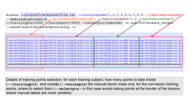
bianca --singlefile=masterfile.txt --trainingnums=1,2,3,4,5,6,7,8,9 --labelfeaturenum=4 \
--querysubjectnum=10 --brainmaskfeaturenum=1 --featuresubset=1,2 --matfeaturenum=3 \
--trainingpts=2000 --nonlespts=10000 --selectpts=noborder -o sub-010/bianca_output \
--saveclassifierdata=mytraining -v

Look at the output

fsleyes sub-010/FLAIR_brain.nii.gz sub-010/bianca_output.nii.gz -cm red-yellow -a 70 &

Since we used the option --saveclassifierdata we also have two additional outputs:

• mytraining: file containing the features derived from the training points
• mytraining_labels: file containing the labels (lesion/non-lesion) for the training points

After running BIANCA

fslmaths sub-010/bianca_output.nii.gz -thr 0.9 -bin sub-010/bianca_output_bin.nii.gz

Masking. To further reduce false positive voxels, we can mask our output. For example, we can exclude areas we are either not interested in (e.g. the cortex), or where BIANCA currently struggles to correctly segment lesions (e.g. subcortical structures and cerebellum).

In this case we prepared such a mask for you: sub-010/prebaked/T1_bianca_mask_to-FLAIR_bin.nii.gz.
Have a look at it on FSLeyes.
How do you apply the mask to the lesion map using fslmaths? Check the command line here.

fslmaths sub-010/bianca_output_bin.nii.gz -mul sub-010/prebaked/T1_bianca_mask_to-FLAIR_bin.nii.gz \
          sub-010/bianca_output_bin_masked.nii.gz

fslmaths sub-010/bianca_output_bin.nii.gz -mas sub-010/prebaked/T1_bianca_mask_to-FLAIR_bin.nii.gz \
          sub-010/bianca_output_bin_masked.nii.gz
  

Add the masked lesion map on FSLeyes and look at the results.

The mask we just used was created using BIANCA side-script make_bianca_mask (more details on the BIANCA documentation page)
Optional extension: to see how to create and apply the mask, click here.

Volume calculation. How would you calculate the volume (in mm³) of the final lesion map using fslstats? Check your answer here.

fslstats sub-010/bianca_output_bin_masked.nii.gz -V

Extension: segment lesions for a new subject with existing BIANCA training file

In the example above, we trained and tested BIANCA within a single call. Since we saved the training files (features and labels) we can apply BIANCA to one (or more) new subject(s) without the need to re-train BIANCA. How would you use BIANCA to segment lesions on a new subject (e.g. sub-011, not present in this dataset), using the training file we obtained above? Consult the BIANCA documentation page if you are unsure. Check your answer here.

echo  sub-011/FLAIR_brain.nii.gz \
      sub-011/T1_brain_to-FLAIR_brain.nii.gz \
      sub-011/FLAIR_brain_to-MNI_xfm.mat \
      sub-011/FLAIR_Lesion_mask.nii.gz >> masterfile_new.txt

  bianca --singlefile=masterfile_new.txt --loadclassifierdata=mytraining --querysubjectnum=1 \
  --brainmaskfeaturenum=1 --featuresubset=1,2 --matfeaturenum=3 \
  -o sub-011/bianca_output -v 

Advanced extension: training and testing with leave-one-out

bianca --singlefile=masterfile.txt --trainingnums=1,2,3,4,5,6,7,8,9 --labelfeaturenum=4 --querysubjectnum=1 \
--brainmaskfeaturenum=1 --featuresubset=1,2 --matfeaturenum=3 \
--trainingpts=2000 --nonlespts=10000 --selectpts=noborder -o sub-001/bianca_output -v

Open the output on FSLeyes, together with the FLAIR image and the manual mask.

bianca_overlap_measures sub-001/bianca_output 0.9 sub-001/FLAIR_Lesion_mask.nii.gz 1

fslmaths sub-001/bianca_output -mas sub-001/prebaked_advanced/T1_bianca_mask_to-FLAIR_bin.nii.gz sub-001/bianca_output_masked.nii.gz
bianca_overlap_measures sub-001/bianca_output_masked 0.9 sub-001/FLAIR_Lesion_mask.nii.gz 1

More details and guidelines for your analysis can be found in the BIANCA documentation.

SIENA (Optional)

SIENA is a package for both single-time-point ("cross-sectional") and two-time-point ("longitudinal") analysis of brain change, in particular, the estimation of atrophy (volumetric loss of brain tissue).

cd ~/fsl_course_data/seg_struc/siena
ls

The example data is two time points, 24 months apart, from a subject with probable Alzheimer's disease. The command that was used to create the example analysis is (don't run this - it takes too long!):

siena sub3m0 sub3m24 -d -m -b -30

The -d flag tells the siena script not to clean up the many intermediate images it creates - you would not normally use this. The other options are explained later.

SIENA has already been run for you. Change directory into the SIENA output directory:

cd sub3m0_to_sub3m24_siena
ls

In the SIENA output directory the first timepoint image is named "A" and the second "B", to keep filenames simple and short. To view the output report, open report.html in a web browser. The next few sections take you through the different parts of the webpage report, which correspond to the different stages of the SIENA analysis.

BET brain extraction results

First BET was run on the two input images, with options telling it to create the skull surface image and the binary mask image, as well as the default brain image.

Other BET options can be included in the call to siena by adding -B "betopts" - for example

siena sub3m0 sub3m24 -d -m -b -30 -B "-f 0.3"

the command line tells siena to pass on the -f 0.3 option to BET, which causes the estimated brain to be larger if the value used is less than 0.5, and smaller otherwise.

You also might need to use the -c option to BET if you need to tell BET where to center the initial brain surface, such as when you have a huge amount of neck in the image. For example, if it looks like the centre of the brain is at 112,110,78 (in voxels, e.g. as viewed in FSLeyes), and you want to combine this option with the above -f option, you would add, to the siena command,

siena sub3m0 sub3m24 -d -m -b -30 -B "-f 0.3 -c 112 110 78"

You can see the two brain and skull extractions in the webpage report. If you want to see these in more detail, open the relevant images in FSLeyes, for example:

fsleyes A A_brain -cm red-yellow A_brain_skull -cm green &

Be aware that the skull estimate is usually very noisy but that it is only used to determine the overall scaling and this process is not very sensitive to the noise as long as the majority of points lie on the skull.

FLIRT A-to-B registration results

Now the two time points are registered using the script siena_flirt. This runs the 3-step registration (brains, then skulls, then brains again). The transformation is "halved" so that each image can be transformed into the space halfway between the two. The webpage report shows the alignment of the two brains in this halfway space. You need to check that the two timepoints are fundamentally well-aligned, with only small (e.g. atrophy) changes between them. Look out for mistakes such as: the two images coming from different subjects, one image being left-right flipped relative to the other one, or one image having bad artefacts.

If you want to look at the registration in more detail:

fsleyes A_halfwayto_B_brain B_halfwayto_A_brain &

FLIRT standard space registration results

Now, if standard-space-based masking has been requested (it was in this case, using the -m option in the command above), the two brain images are registered to the standard brain $FSLDIR/data/standard/MNI152_T1_2mm_brain using FLIRT. The transforms (and their inverses) are saved. The two brains are registered separately and their transforms compared to test for consistency.

The webpage report shows the two images transformed into standard space, with the overlaying red lines derived from the edges of the standard space template, for comparison.

Field-of-view and standard space masking

If the -m option was set, a standard space brain mask is now transformed into the native image space and applied to the original brain masks produced by BET. This is in most areas a fairly liberal (dilated) brain mask, except around the eyes.

If the -t or -b options are set then an upper or lower limit (in the Z direction) in standard space is defined, to supplement the masking. This is useful, for example, to restrict the field-of-view of the analysis if you have variable field-of-view at the top or bottom of the head in different subjects.

Here you can see the bottom of the temporal lobes have not been included in the regions fed into the boundary edge movement analysis. You would use such a setting if these regions had not been acquired in one/some of the subjects in your dataset.

The webpage report shows the -m brain masking in blue, the -t/-b masking in red (you can see the effect of the -b -30 option), and the intersection of the two maskings in green. It is this intersection that is what gets finally used.

FAST tissue segmentation

In order to find all brain/non-brain edge points, tissue-type segmentation is now run on both brain-extracted images. The GM and WM voxels are combined into a single mask, and the mask edges (including internal ventricle edges) are used to find edge motion (discussed below). The webpage report shows the two segmentations.

Change Estimation

The final step is to carry out change analysis on the registered masked brain images. At all points which are reported as boundaries between brain and non-brain, the distance that the brain surface has moved between the two time points is estimated. The mean perpendicular surface motion is computed and converted to PBVC (percentage brain volume change).

The webpage report shows the edge motion colour coded at the brain edge points, and then shows the final global PBVC value. To see the edge motion image in more detail:

fsleyes A_halfwayto_B_render -cm render1 &

"LOOK AT YOUR DATA" - SIENA Problem Cases

We now look at 4 examples of "problem cases" - these were real cases that occurred in one study; they illustrate some of the problems/mistakes that sometimes occur.

Example 1

cd ~/fsl_course_data/seg_struc/siena_problems/eg1/S2_032_ax_to_S2_164_ax_siena

Open report.html in a web browser.

Look at the FLIRT A-to-B registration results. Can you tell what's wrong? If you're unsure, click here.

Example 2

cd ~/fsl_course_data/seg_struc/siena_problems/eg2/S2_039_ax_to_S2_142r_ax_siena

Open report.html in a web browser.

Look at the FLIRT A-to-B registration results. Can you tell what's wrong? If you're unsure, click here.

Example 3

cd ~/fsl_course_data/seg_struc/siena_problems/eg3/S2_080_ax_to_S2_121_ax_siena

Open report.html in a web browser.

Look at the FLIRT A-to-B registration results. Can you tell what's wrong? If you're unsure, click here.

Example 4

cd ~/fsl_course_data/seg_struc/siena_problems/eg4/S2_002_ax_to_S2_162_ax_siena

Open report.html in a web browser.

Look at the FLIRT A-to-B registration results. Can you tell what's wrong? If you're unsure, click here.

SIENAX (Optional)

cd ~/fsl_course_data/seg_struc/siena/sub3m0_sienax

In this section we look at how SIENAX works and look at the most useful outputs. SIENAX estimates total brain tissue volume, from a single image, normalised for skull size.

Open report.html in a web browser. The example data is one time point from a subject with probable Alzheimer's disease. The command that was used to create the example analysis is (don't run this!):

sienax sub3m0 -d -b -30 -r

SIENAX starts by running BET and FLIRT in a manner very similar to SIENA, except that the second time point image is replaced by standard space brain and skull images. Next a standard space brain mask is always used to supplement the BET segmentation.

As before, optional Z limits in standard space can be used to mask further.

Next, FAST is used, with partial volume estimation turned on, to provide an accurate estimate of grey and white matter volumes. In order to provide normalised volumes for GM/WM/total, the volumetric scaling factor derived from the registration to standard space is used to multiply the native volumes; the values are thus normalised for head size.

FIRST Revisited (Optional)

Uncorrected segmentation output

cd ~/fsl_course_data/seg_struc/first

This follows on from the initial part of the FIRST practical above and assumes that run_first_all has been successfully run. Having considered the boundary corrected segmentation previously, we now turn to look at the uncorrected segmentation.

The uncorrected segmentation shows two types of voxels: ones that the underlying surface mesh passes through (boundary voxels) and ones that are completely inside the surface mesh (interior voxels). FIRST uses a mesh to model the structure when doing the segmentation, so converting this to a volume requires it to be split into boundary and interior regions like this.

We will now look at the uncorrected volumetric segmentations:

fsleyes con0047_brain con0047_all_fast_origsegs &

To view the segmentation better change the colourmap of the segmented image to Red-Yellow and make the Max display range value to 100 for this image. Note that you see the interior voxels and the boundary voxels in different colours. This is because the boundary voxels are labeled with a value equal to 100 plus that of the interior voxels. That is, the interior and boundary voxels for the left hippocampus are labeled 17 (the CMA label designation for left hippocampus) and 117 respectively.

The volume con0047_all_fast_origsegs is a 4D file containing each structure's segmentation in a separate 3D file. If you change the Volume control on FSLeyes to go from 0 to 1 then you will see the left amygdala result. These are separated in case these uncorrected segmentations overlap. Play with the opacity settings (or turn the segmentation on and off) to see how good the segmentation is.

These images require boundary correction which is done automatically by run_first_all. However, there are alternative methods for doing the boundary correction which you can specify with run_first_all or as a post-processing on the uncorrected image with first_boundary_corr, although the settings used by run_first_all have been chosen as the optimal ones based on empirical testing.

Multi-Channel FAST (Optional)

cd ~/fsl_course_data/seg_struc/fast

Multi-channel segmentation is useful for when the contrast or quality of a single image is insufficient to give a good segmentation. Typically, this type of segmentation is not needed for healthy controls with good T1-weighted images, as the single channel results are good and are often even better than the multi channel results. However, when pathological tissues/lesions are present, or when the T1-weighted image quality is not good, multi-channel segmentation can take advantage of the extra contrast between tissue types in the different images and give better results.

In sub2_t1 and sub2_t2 are T1-weighted and T2-weighted images of the same subject. Are they well aligned? You can get an easy non-interactive combined view of two images (which must have the same image dimensions) with slices:

slices sub2_t1 sub2_t2

They look reasonably aligned in sagittal and coronal view, but axial views clearly show misalignment between scans (if you cannot clearly see the axial slices, open the same two images in FSLeyes). Before running multi-channel FAST it is necessary to use FLIRT to register the data. Start by running Bet on each image to remove the non-brain structures, producing subj2_t1_brain and sub2_t2_brain. Note that it is OK if one of the brain extraction results includes non-brain matter (e.g. eyeballs) but the other is accurate, since the brain mask used by FAST will be the intersection of the two masks.

Start the FLIRT GUI:

Flirt &

For this example use the following settings:

• Reference image: sub2_t1_brain (clear the existing directory name in the file browser and press enter to get to the local directory).
• Input image: sub2_t2_brain
• Output image: sub2_t2_to_t1
• DOF: 6

Load sub2_t1_brain and sub2_t2_to_t1 into FSLeyes to check the result of the registration. Change the colour map for the higher image in the list to Red-Yellow and increase its transparency so that you can see how good the overlap is.

You can now forget sub2_t2.

Run Fast (with the Number of input channels set to 2) on the multi-channel brain-extracted images sub2_t1_brain and sub2_t2_to_t1_brain (or whatever you called these BET outputs). Asking for the default number of classes (3 - assumed to be GM/WM/CSF) gives poor results because bits of other tissues outside of the brain are given a class - so you should run with 4 classes; then results should be good. This takes a few minutes; move on to the next part of the practical and view the results once fast has finished running.

Advanced: FAST - Other Options

If you have time to spare after finishing the other practical parts then you can come back and test the effect of various FAST options, obtained by typing:

fast -h

You could also work out how to colour-overlay segmentation results onto the input image using the overlay command.

The End.