Winkler AM, Ridgway GR, Douaud G, Nichols TE, Smith SM
Neuroimage. 2016;141:502-516. (Open Access)
http://dx.doi.org/10.1016/j.neuroimage.2016.05.068
In the pages with the plots, each row is a repetition with a different number of permutations, and each column is a repetition varying a parameter for each case. Not all methods have a parameter to vary (these have just one column, titled "NaN"), and not all methods can be performed with a varying number of permutations (these have just a single row).
The PP and QQ plots are shown in log-scale, whereas the Bland–Altman plots are shown in the usual linear scale. The PP plots have in the horizontal axis the p-value for the reference set (50k shufflings), and the vertical axis for the method being tested. The QQ plots are similar, but have all values sorted, such that they correspond to the ranks (true QQ plots would need the expected values in the horizontal axis and here we take the 50k as equivalent to the expected; this is needed because TFCE does not have a uniform distribution under the null). The BA are modified so as to use in the horizontal axis not the average of the two p-values, but the one using the reference set.
The shaded regions for all these plots correspond to the 95% confidence interval: for the PP, the CI is plotted around the identity line, whereas for the QQ, it is ploted around the respective dots. For the BA, it is the CI for the difference, with the ellipsoid shape.
The multivariate tests used were Wilks' \(\lambda\) (W) and Pillai's trace (P). For the NPC, the letters indicate Tippett (T) and Fisher (F).
In the pages linked below the terms EE and ISE refer to assumptions about the error terms: EE stands for exchangeable errors (that allows permutations), ISE for independent and symmetric errors (that allow sign flippings) and EE+ISE allows both types of shuffling simultaneously.
Note: For the tail and gamma approximations, for the case in which the non-permuted statistic was left out of the empirical distribution (T1out), some of the log(QQ) plots seem to show p-values in the x-axis (reference set) that do not seem to reach the upper limit of -log(50k)=4.7. The reason for this apparent discrepancy is that, particularly for the cases in which few permutations are used, many accelerated p-values are found as identical to zero, which lead to -log(0)=Inf, and thus, cannot be paired with the reference set for the scatter plot. This is not merely an artefact, and can be read as evidence favouring the inclusion of the non-permuted statistic in the null distribution.
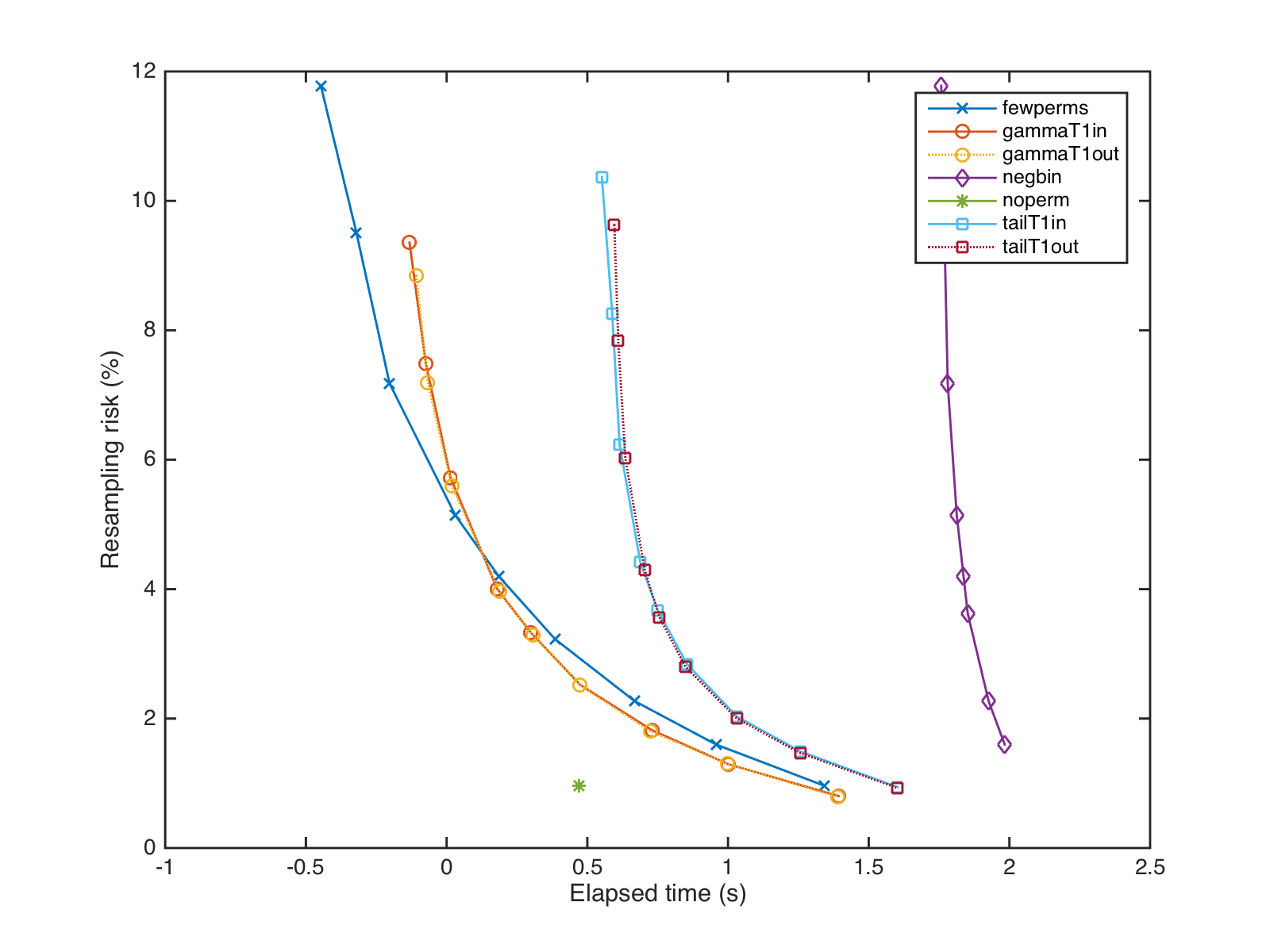
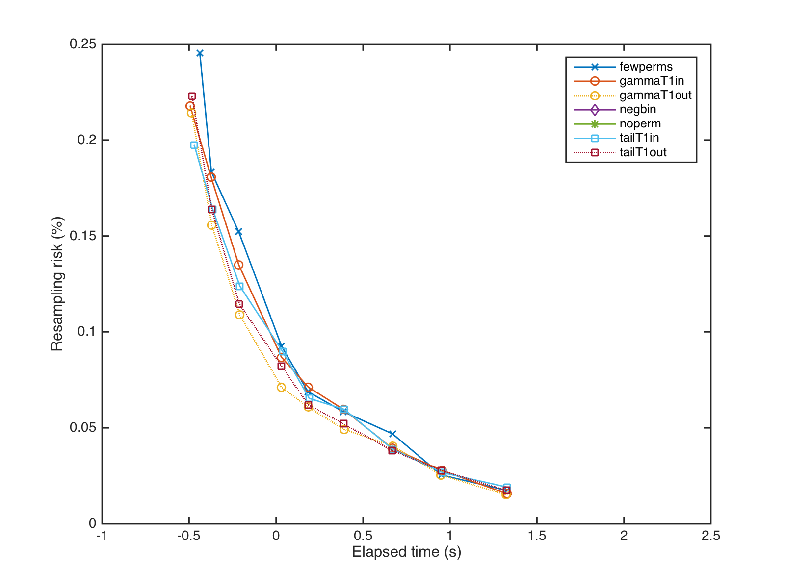
In addition, for the univariate, Gaussian errors, with and without signal, and exchangeable errors (permutations only), 100 realisations were performed using the various parameters, thus allowing empirical standard deviations (as opposed to confidence intervals) and histograms to be plotted, as well as to estimate the resampling risk. The timings are shown in seconds, and refer to runs of PALM using simple voxelwise results (i.e., no spatial statistics), such that they are comparable.
| Without signal | With signal | |
|---|---|---|
| Plots | click here | click here |
| Rates | click here | click here |
| Timings | click here | click here |
Note: The timings refer to uncorrected voxelwise results; for tail and gamma approximations, the extra time needed only for the FWER correction is negligible.
Plots for the trade off between speed and resampling risk, showing curves also for the tail and gamma approximations when the unpermuted statistic is included in the null distribution are here: [ uncorrected | corrected ]
Below are the results of running the various methods on the same dataset used for the TFCE paper, with two different levels of smoothing.
| \(\sigma\) = 3 mm | \(\sigma\) = 6 mm |
|---|---|
| click here | click here |
Note: The two \(\sigma\) values were only to assess the overall effect of smoothing, and should not be interpreted as recommendations on smoothing levels for VBM analyses. This is particularly the case for \(\sigma\) = 6 mm.