newMSM user guide
Introduction
Before reading this guide, it is strongly recommended to read the original MSM user guide, because the fundamental operation remained the same. Some of the theoretical background and basic usage are described there. In this guide, we outline improvements in the optimisation method and regularisation, along with several new features.
Method improvements
Optimisation
The discrete cost function is as follows:
This is a Markov Random Field (MRF) cost which seeks to assign labels to each data point so as to maximise some estimate of data likelihood whilst penalising sharp changes in labelling points between neighbouring points. Thus, the cost function balances a data similarity term, \(\rho_{p} (l_{p})\), which estimates the overlap of features for that proposed move, with a regularisation penalty, \(W_{pqr} (l_{p},l_r,l_s)\), which penalises the hyper-elastic strain energy of the resulting deformation (described in detail later).
Most often for MSM similarity is assessed through cross-correlations, either for overlapping image patches, or (if you are using multiple feature maps) an average of correlations of feature vectors at each corresponding point in space.
When finally estimated discrete displacements of the control point grid are then upsampled (or interpolated) to the original sphere using barycentric interpolation to get the final warp.
Cliques
In discrete optimisation cliques are groups of data points, for example they can be single \(\{p\}\), pairs \(\{p,q\}\), triplets \(\{p,q,r\}\) or higher orders. In MSM the highest we go to is 3 and this reflect triplets of points, reflecting the vertex corners of each triangular face in the mesh.
In the first version of MSM (pre-2018) the highest order of clique considered is two. This reflects the fact that standard discrete optimisation libraries optimise MRFs where the maximum clique size is two (pairs); this is largely due to the significant computational challenges involved in programming approximations that work for such increasingly complex combinatorial problems. The issue with this is it only allows first-order smoothness penalties - i.e. you can only look at the rate of change of displacement between neighbouring points \(\{p,q\}\). Most successful modern registration aim to penalise second order effects using, for example, bending energy penalties.
MSM_HOCR regularisation
HOCR stands for Higher Order Clique Reduction, which is based on work done by Hiroshi Ishikawa (Ishikawa, 2014) in which algorithms were proposed which reduce higher (than 2) order clique terms to a linear combination of pairwise and univariate terms through polynomial approximation. This allows higher-order MRFs to be solved with standard MRF solvers such as Fast-PD (as used by the original MSM). This allows MSM to move from using a fairly weak pairwise penalty to a tri-order biomechanical strain based regularisation:
This penalises both scale \(J=\lambda_2\lambda_2\) and shape \(R=\lambda_1/\lambda_2\) distortions of the triangles of the control-point mesh, where \(\lambda_1\) and \(\lambda_2\) are the principal stretches or eigenvalues of the 2D deformation tensor \(\mathbf{F_{pqr}}\) and the bulk (\(\kappa\)) and shear (\(\mu\)) moduli are parameters which weight the relative importance of the two terms.
New features
Anatomical MSM
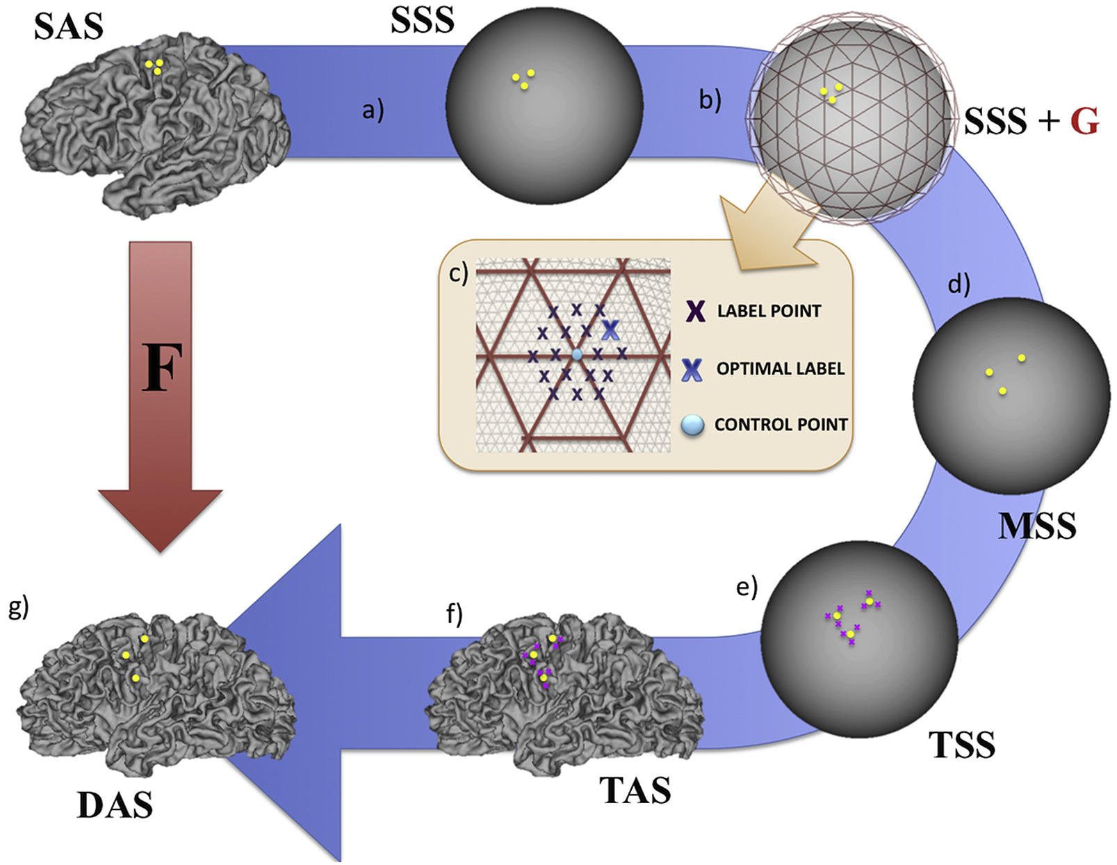
Strain based regularisation has proved extremely vital for improving quality of alignment for noisy datasets such as fMRI. However, this is not it's only benefit. It can also be used to indirectly infer a smoothed and regularised mapping of the cortical anatomy.
Here, warps continue to be inferred between source and targets spheres (SSS and TSS) via displacements of points to discrete locations defined on the sphere. However, due to one-to-one correspondence between vertices for each subject's sphere and (white/pial/midthickness) surface, it means it is possible to infer an anatomical warp (SAS, DAS) by projecting the moving surface mesh topology (SAS) onto the target anatomical surface (TAS) shape, using the location of source vertices (shown in yellow) relative to target vertices (shown in pink: TSS) to perform the weighted (barycentric) resampling. This leads to a deformed configuration of the source anatomy (DAS) where the 2D transformations (\(\mathbf{F_{pqr}}\)) of mesh faces (from SAS-DAS) can then be regularised using biomechanical strain (\(\mathbf{W_{pqr}}\)).
If you seek to run aMSM and penalise anatomical deformations you might consider the following options:
--anatgrid- this uses a downsampled version of the anatomical grid to estimate the distortions \({F_{pqr}}\). The downsampled meshes are estimated through projection of different icospheric mesh resolutions onto the anatomical surface. We found that going lower than ico 3 downgraded performance and advise starting with 4.
In general the command line calls will remain exactly the same. The exception being when you want to run aMSM. Here, you need to supply the input and target cortical anatomy files using the --inanatand --refanat options. Here, the anatomy can be the white, pial, midthickness (or even inflated) surfaces. Each will place different constraints on the alignment. An example call to aMSM is as follows:
newmsm \
    --inmesh=input_sphere.surf.gii \
    --refmesh=ref_sphere.surf.gii \
    --inanat=input_midthickness.surf.gii \
    --refanat=ref_midthickness.surf.gii \
    --indata=in_data.func.gii \
    --refdata=ref_data.func.gii \
    --out=~/mydirname/L. \
    --conf=aMSM_strainconf \
    --verbose
For more guidance on the impact of parameter choices for aMSM, and guidance on applying to your data please refer this paper. If you are expressly interested in Biomechanical modelling, detailed optimisation and configuration guidance is supplied in the supplementary information of Garcia et al, 2018, where aMSM was used to build a model of cortical growth in preterm neonates.
Groupwise MSM
We extended the existing MSM framework to perform groupwise registration by simultaneously co-registering clusters of surfaces, which share common modes of cortical variation. Let's say, there exist \(n\) moving meshes for any given cluster; each input surface is therefore associated with its own low-resolution CP grid. For each iteration, the groupwise registration must choose the optimal discrete displacement for all CP grid by comparing the overlap of features, across all inputs, for the set of proposed moves. For each CP grid, this involves calculating the similarity between overlapping patches of features, defined around each of its CP vertices, and all overlapping patches defined for neighbouring vertices in all other CP grids. These are defined by propagating the proposed mapping to the resolution of the input feature maps, and resampling all data to a common reference frame (\(F\)) to calculate patch overlap. Here \(F\) is defined from a high resolution icospheric tessellation (ico6 - 40,962 vertices), and features are resampled using adaptive barycentric interpolation. Regularisation is then implemented by calculating the hyper-elastic strain of every proposed move on all subjects' CP grid. Then, the energy function to minimise is:
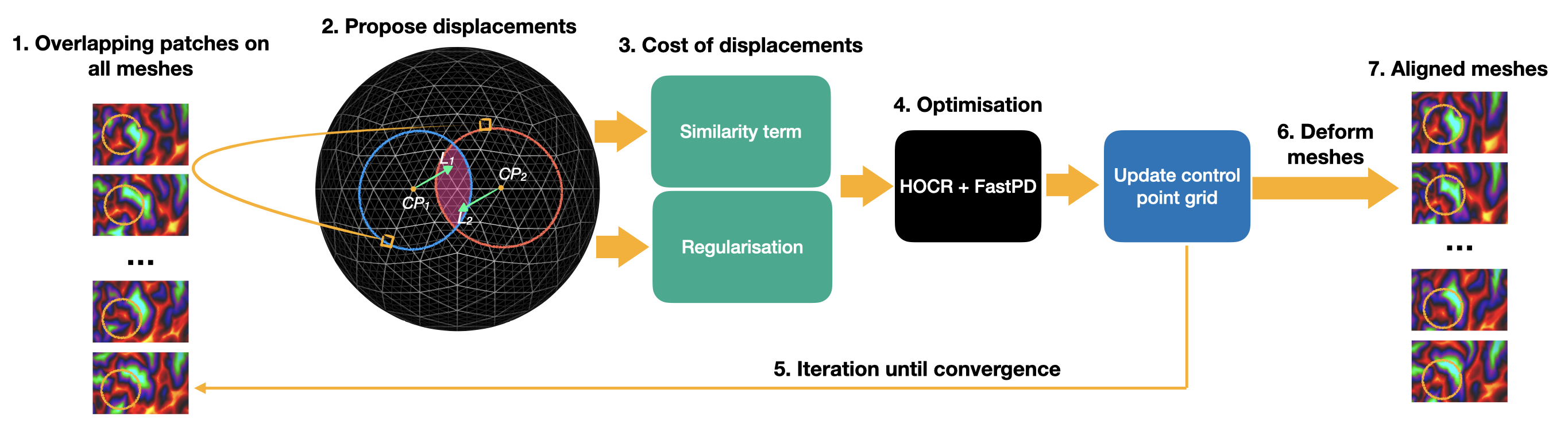
The figure above shows the overview of the groupwise registration process. The input of the method is pairs of overlapping patches on all meshes across the group (step 1). These patches are moved around the labels (2), then the calculated costs of all displacements (3) are minimised by the optimisation method (4). Then all CP grids are updated. This iteration runs until convergence (5), then all meshes are deformed (6) according to the results of the optimisation. The aligned meshes (7) then resampled to the output space and saved. As an example, yellow circles highlight patches that are aligned during the process from step 1 to 7. Blue and red circles denote patches on different subjects, similarity costs are calculated on the overlapping area of patches.
Configuration files in newMSM
Configuration files modify all tunable parameters of the registration. For a full list of all registration parameters you can enter: newmsm -p.
Some parameters require inputs for every stage of the registration, and are input as comma separated lists e.g. --lambda=0,0.1,0.2,0.3 (for four levels). These are:
--lambdaweights the contribution of the regulariser relative to the similarity force.--optselects the optimisation approach. Choice of:AFFINEorDISCRETE(default)--simvalselects the similarity measure for each stage of the registration. There is a choice of 1) SSD; 2) correlation (default) or 4) DICE overlap. For discrete optimisation we strongly recommend correlation for all datasets. The current implementations of SSD does not in general work well in the discrete case, and we do not advise using it.--itcontrols the maximum number of iterations at each resolution. In general affine registration will require in excess of 30 iterations. Discrete optimisation usually converge after 5-10 iterations.--sigma_insets the input smoothing: this changes the smoothing kernel's standard deviation (default--sigma_in=2,2,2, but for very noisy data we suggest you smooth more)--sigma_refsets the reference smoothing: the values are equal tosigma_inby default, but you could smooth the reference less than the input if you are using an average template.--datagridin MSM data is typically downsampled from the high resolution surfaces input mesh and reference mesh onto a regular (equally spaced vertex) grid. This speeds up the running of MSM without appreciably downgrading the quality of the alignment. These grids are formed from subdivision of a icosahedron and are coded in terms of the number of resamplings performed. For datagrids we typically we use 10K grids, which have code 5.--CPgridthe Control Point (CP) Grid is a low resolution mesh that controls the warp of the input mesh to the reference. At each iteration of the registration, the CP Grid can undergo one of a discrete set of deformations, where end points are defined by points on the sampling grid. By default the first level of the discrete optimisation is started with a 162 vertex grid (code 2) and this is increased by one for each level. Lower resolution CP grids move larger data patches for large distances, whilst higher resolution ones move smaller data patches for smaller distances.--SGgridthe Sampling Grid resolution determines the maximum number of discrete deformations available to each CP and thus the maximum possible accuracy of the registration at that stage of the registration. It is set 2 levels higher than the CP resolution by default.
Other parameters need only be specified once:
--excltells MSM to ignore an 'exclusion' region; defined by thresholding (the intensity range provided by the cut threshold below)--cutthrcontrols the exclusion region, which is defined for all intensities between a certain intensity range. It needs two values as upper and lower thresholds for defining cut vertices. As it is usually used to mask the cut on the medial wall (which is zero valued) these values are typically--cutthr=0,0.0001--INused to normalize the intensity range of the target to that of the input data using histogram matching--VNused to variance normalize input data across all channels--regoptionused to set the regulariser. Only strain based regularisation is available. Set this value to 3 for typical and groupwise MSM and 5 for anatomical MSM.--doptused to select optimiser. Possible values areFastPDorHOCR. As an experimental feature,MCMCcan be selected.--tricliqueoption to calculate correlation on mesh face triangle patches instead of circular patches around a CP grid vertex.--shearmodshear modulus and--bulkmodbulk modulus. Investigations in the 2018 MSM paper showed that a) this default parametrisation worked for adult and neonatal brains and b) the method was robust to a range of choices of values. There should be no reason to change from these default values unless you want to do advanced biomechanical modelling of the type described in Garcia et al, 2018.--k_exponentk exponent. See regularisation section in 2018 NeurImage paper.--regexpregularisation exponent. See regularisation section in 2018 NeurImage paper.--rescaleLthis argument updates the discrete label space at each iteration to allow more thorough sampling of the entire space (for more details see this paper. It makes the process run slower but improves performance.--cprangeincrease or decrease the range of sampling from the control point.--stepsizeaffine registration parameter.--gradsamplingaffine registration parameter.--numthreadsnumber of execution threads. newMSM can run on multiple CPU threads. (Default is 1)--mcitersnumber of Monte Carlo iterations. See Markov Chain Monte Carlo optimiser section.--mcparamparameter for the random number generator. See Markov Chain Monte Carlo optimiser section.--patchwisecalculating similarity patchwise instead of featurewise in multimodal mode.--percentilethresholding percentile for DICE overlap similarity metric. (Default is 0.75)--fixnanFixing NaN cost function results with the value 1e7.
An example configuration file is:
--simval=1,2,2,2
--sigma_in=2,4,2,1
--sigma_ref=2,2,1,1
--lambda=0,0.2,0.2,0.2
--it=50,20,25,25
--opt=AFFINE,DISCRETE,DISCRETE,DISCRETE
--CPgrid=0,2,3,4
--SGgrid=0,4,5,6
--datagrid=4,4,5,6
--regoption=3
--regexp=2
--dopt=HOCR
--IN
--k_exponent=2
--bulkmod=1.6
--shearmod=0.4
--rescaleL
The comma separated lists above represent parameters per level, and the number of resolution levels run by MSM can be controlled by the length of the lists specified here. Registration may also be initialised using an affine alignment step, run as an additional level at the beginning. Therefore, the above case is stating that the registration should run one affine step using: SSD as a similarity measure, 50 iterations, input mesh smoothing 2mm, reference mesh smoothing 2mm, on a data grid of resolution 2562 vertices. Following this, discrete optimisation is run over 3 levels with 3 iterations at each level, using control point grid resolutions 162, 642, and 2562, where the sampling grid resolution is 2 subdivisions above this, and the data grids have resolution: 2562, 10242 and 40962 vertices. Smoothing is applied to the source image as 4, 2, then 1mm sigma smoothing kernels, and to the reference image as 2, 1 and 1mm smoothing. --IN indicates that the source intensity distribution is matched to the target intensity distribution using histogram matching, once at the beginning of the registration.
If you choose to edit or optimise the config files then it is important to remember that all multiresolution level parameter lists must have the same length, else the program will throw the error: MeshREG ERROR:: config file parameter list lengths are inconsistent.
In addition, as affine registration only implements the following parameters: --opt, --simval, --it, --sigma_in, --sigma_ref, --IN, --VN, --scale, --excl, for all other multi level parameters, it is necessary to supply a zero value for the AFFINE stage (see example line --lambda first parameter).