newMSM tutorials

Groupwise registration

In this tutorial, we will guide you through a series of steps to show you how the groupwise mode of MSM works. We will use examples from the HCP dataset, so you should have a few subjects' data downloaded and surfaces reconstructed (with e.g., HCP minimal processing pipeline or Freesurfer).

As a demonstration, to assist the process, we provide pipeline scripts that can be found at GitHub. In this, the gw_MSM.sh script prepares the data, performs registration and post-processes the results. The input of the script is a clustering CSV file that contains a list of subject IDs and corresponding group IDs as demonstrated in the following example (CSV header: line_number, subject ID, group ID):

1,212419.R,NODE1910
2,127933.R,NODE1910
3,135629.R,NODE1910
4,130720.L,NODE1951
5,176239.R,NODE1951
6,221319.R,NODE1951
7,139637.R,NODE1951
8,130114.L,NODE1951
9,130114.R,NODE1951
...

NODE1910 and NODE1951 are groups that contain subjects 212419.R, 127933.R, etc.

In the bash script file you can set: - the input folder where your data resides, - a work directory where the outputs and results will be saved, - the clustering CSV file path, - the template (i.e. registration output space) file path, - the configuration file path, - and the group ID you want to register.

The required arguments of newmsm are: - data: the list of data files (created by the script), - meshes: the spherical meshes that the data is on (created by the script), - template: the output space of the registration, - conf: config file (will be detailed later), - out: output path and file name prefix, - groupwise: required to start MSM in groupwise mode.

Optional arguments are: - verbose: more state messages printed to the console output, - mask: this will set a weight mask to all meshes.

Example:

$HOME/fsldev/bin/newmsm \
  --data=$workdir/file_lists/input_data_$group_id.txt \
  --meshes=$workdir/file_lists/input_meshes_$group_id.txt \
  --mask=$workdir/configs/maskfile.func.gii \
  --template=$template \
  --conf=$config_file \
  --out=$outdir/$group_id/groupwise.$group_id. \
  --verbose --groupwise

There are a few differences that you should consider when you set your config files. In general, you might need to set the regularisation (lambda) somewhat higher than in typical MSM. In the case of sulcal depth or curvature, this means somewhere between 0.2-0.5. All similarity metrics are available, but we recommend using the Pearson's correlation coefficient (simval=2). For the optimiser, only HOCR is available (MCMC is being developed) and triclique likelihood, the rescaleL option and anatomical mesh regularisation are not available (so use regoption=3). Also note that AFFINE registration is not available at the moment, so it is advised to perform affine alignment separately to a template before groupwise registration (usually this step is done before clustering). Parallelisation is available. As a new option, --fixnan can change NaN values to 1e7, providing more stability to the FastPD optimiser.

An example config file:

--simval=2,2,2
--sigma_in=0,0,0
--sigma_ref=0,0,0
--lambda=0.2,0.2,0.2
--it=9,9,9
--opt=DISCRETE,DISCRETE,DISCRETE
--CPgrid=2,3,4
--SGgrid=4,5,6
--datagrid=4,5,6
--regoption=3
--regexp=2
--dopt=HOCR
--k_exponent=2
--bulkmod=1.6
--shearmod=0.4
--numthreads=4

After registration, we apply dedrifting for the outputs of the registration for the entire group. We calculate the surface average of the inverse registration and correct all outputs. Finally we generate mean and standard deviation maps and areal and shape distortion maps.

The most important outputs of the pipeline consists of the following files:

• groupwise.$group_id.sphere-$subject_id.reg.corrected.surf.gii: the dedrifted mesh
• groupwise.$group_id.sphere-$subject_id.distortion.func.gii: distortion map of subject
• groupwise.$group_id.transformed_and_reprojected.dedrift-$subject_id.func.gii: aligned data
• groupwise.$group_id.areal.distortion.merge.sulc.affine.dedrifted.ico6.shape.gii: areal distortion of all subjects
• groupwise.$group_id.shape.distortion.merge.sulc.affine.dedrifted.ico6.shape.gii: shape distortion of all subjects
• groupwise.$group_id.mean.sulc.curv.affine.dedrifted.ico6.shape.gii: mean maps
• groupwise.$group_id.shape.distortion.merge.sulc.affine.dedrifted.ico6.shape.gii
• groupwise.$group_id.stdev.curv.affine.dedrifted.ico6.shape.gii: standard deviation map of all subjects

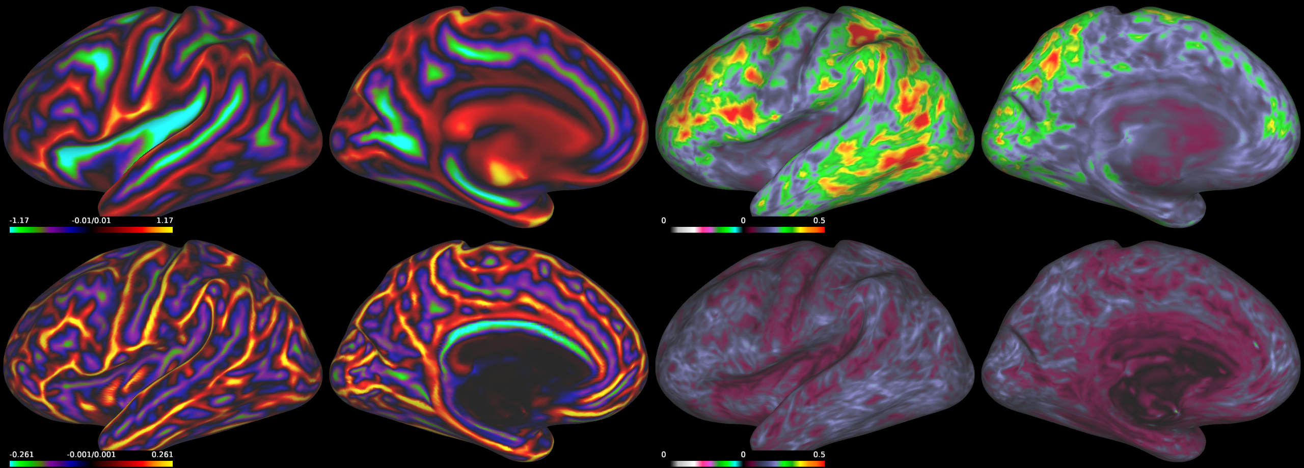
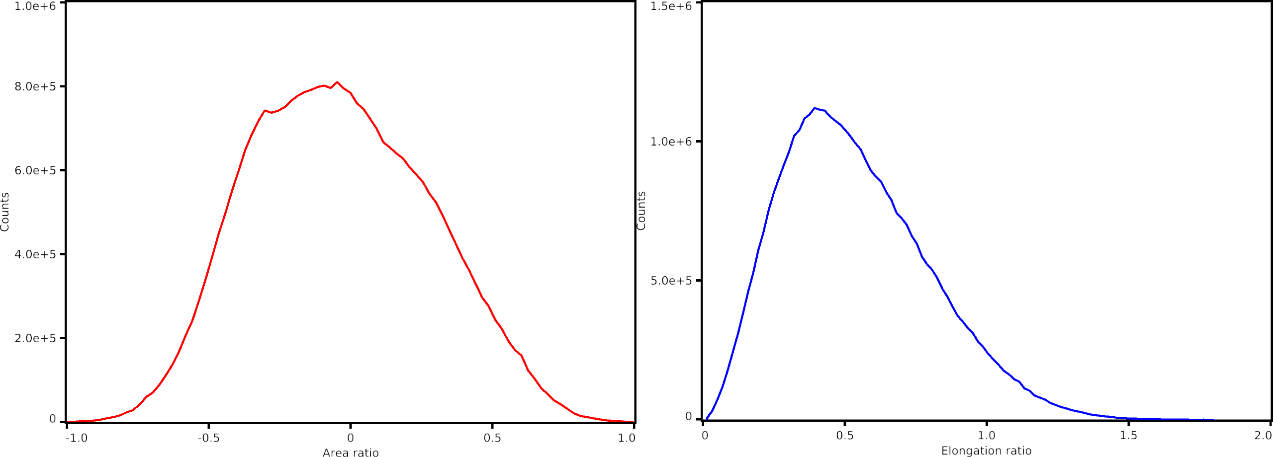
The figures below illustrate the output of the pipeline. First figure (from top left to bottom right): sulcal depth mean, sulcal depth standard deviation, curvature mean and curvature standard deviation maps. Second figure (from left to right): areal distortion and shape distortion charts.

As an optional step, we show how we compared gMSM results with typical registration. For this we provide the typical_MSM.sh and compare_stats.py scripts. The typical_MSM script performs "typical" registration (i.e. individual subject to template), so you will need to choose a template. In the script provided, this template is MSMStrain.L.sulc.curv.ico6.shape.gii. After registering all the subjects in the specified group to the same template, we generate the mean, standard deviation and areal and shape distortion maps, just as we did with the groupwise results. After this, the compare_stats.py script calculates cross-correlation similarity (pairwise average), DICE overlap ratio (percentile can be changed, .75 is the default) and different areal and shape distortion statistics, as shown below for NODE2078:

Stats for group NODE2078
Sulc
    CC similarity: 0.8011; Dice overlap: 0.67
    CC similarity: 0.722; Dice overlap: 0.6028
Curv
    CC similarity: 0.5337; Dice overlap: 0.5684
    CC similarity: 0.2469; Dice overlap: 0.4056
Distortion
    Areal mean: 0.2604; Areal Max: 1.209; Areal 95%: 0.587; Areal 98%: 0.6701; Shape mean: 0.544; Shape Max: 1.801
    Areal mean: 0.1707; Areal Max: 0.6959; Areal 95%: 0.3755; Areal 98%: 0.4272; Shape mean: 0.4109; Shape Max: 1.69